Week 11: Ground Control to Major Progress
May 8, 2026
Hi there, and thanks for stopping by again for the second-to-last week of my senior project! This week, I can confidently say that we’ve made some major progress. If you recall, we unfortunately ended with an error in my code last week. But as they all say, you need a little bit of darkness to see the light. That certainly is true, for this week, the light at the end of the tunnel has become much brighter. I won’t hold the good news from you any longer, so let’s get right into it!
One Error Later
First things first, we have to fix the error from last week. The rather long error code looked like this:
------------------------------------------------------------
ValueError                 Traceback (most recent call last)
Cell In[9], line 52
     39 rf_aligned, rf_proba, rf_std, rf_counts =
     40 align_repeated_summary_to_train_df(
     41     train_df=train_df,
     42     agg_df=rf_oof,
     43     prob_cols=PROB_COLS,
     44     model_prefix="rf",
     45 )
     46 cb_aligned, cb_proba, cb_std, cb_counts =
     47 align_repeated_summary_to_train_df(
     48     train_df=train_df,
     49     agg_df=cb_oof,
     50     prob_cols=PROB_COLS,
     51     model_prefix="cb",
     52 )
---> 53 validate_repeated_counts("RandomForest", rf_counts,
     54 expected_counts)
     55 validate_repeated_counts("CatBoost", cb_counts,
     56 expected_counts)
     57 print("=== Data status ===")

Cell In[8], line 148
    146 mismatch = np.where(observed != expected)[0]
    147 first = mismatch[:10]
---> 148 raise ValueError(
    149     f"{model_name}: repeated-CV validation counts disagree
    150     for {len(mismatch)} sources. "
    151     f"First mismatches at rows {first.tolist()}:
    152     observed={observed[first].tolist()}
            expected={expected[first].tolist()}"
    153 )

ValueError: RandomForest: repeated-CV validation counts disagree
for 2877 sources.
First mismatches at rows [0, 1, 2, 3, 4, 5, 6, 7, 8, 9]:
observed=[1, 1, 1, 1, 1, 1, 1, 1, 1, 1]
expected=[10, 10, 10, 10, 10, 10, 10, 10, 10, 10]
The final few lines indicate that the error arises from a mismatch in the repeated cross-validation (CV) counts. This is because last week, we fixed how we calculated the held-out predictions: rather than overwriting predictions in every repeat, we aggregated all predictions and averaged at the end. However, we didn’t do that originally for our baseline models, so they don’t follow the corrected scheme. This means they have a single prediction value (observed=1 in the error message) rather than one prediction for every repeat (expected=10 in the error message).
At this point, I really only had two solutions. I could either completely retrain both baseline models with the corrected prediction calculation, or I could simply change how I compared the models. I didn’t want to take any shortcuts, so I decided to retrain the baseline models, as tedious as it seemed. After retraining and saving the new aggregated predictions, I successfully loaded the baseline results into my code and proceeded to train the improved Bayesian neural network (BNN).

A Not-So-Starbucks Refresher
Since I’ve already described all of the fixes we’re making in this new BNN iteration in last week’s post, I won’t go into detail this time. I’ll just provide a brief list of all the improvements for a quick recap.
Missing data: Previously, we median-imputed Block B but didn’t expose missing data or values. For tabular data, the fact that a value is missing can carry information. Here we keep the imputed/scaled values and pass binary “missingness” indicators to the network.
Feature-wise embeddings: Instead of feeding standardized scalars directly into one dense layer, we’re embedding each numerical feature separately and only then mixing them in the shared trunk.
Correct repeated-CV aggregation: The earlier iteration overwrote predictions fold by fold. Here, we fix it by aggregating and averaging both the repeated-CV predictive mean and the uncertainty.
Model reconstruction: Of course, the biggest change we made last week was reconstructing the entire model. Rather than the computationally expensive, three-model architecture, we’ve produced a shared-trunk hierarchical BNN. This only requires one model but still includes a robust hierarchical strategy with Bayesian branches in the final layers.
Drumroll for the Results
After making the aforementioned changes, I’ve arrived at some very promising results! As always, let’s compare the evaluation metrics of the new BNN to those of the baseline models and the old BNN. The table below shows the six metrics we’ve become familiar with over the past several weeks:
| Accuracy | F1 | ROC-AUC | NLL | Brier | ECE | |
|---|---|---|---|---|---|---|
| Retrained RF | 0.8495 | 0.8419 | 0.9522 | 0.4276 | 0.0442 | 0.0475 |
| Retrained CB | 0.8442 | 0.8429 | 0.9507 | 0.4273 | 0.0446 | 0.0126 |
| Old BNN | 0.7810 | 0.7762 | 0.9328 | 0.5450 | 0.0570 | 0.0285 |
| New BNN | 0.8443 | 0.8466 | 0.9541 | 0.4485 | 0.0459 | 0.0184 |
From this table, we can clearly see that the repaired BNN has made some considerable progress! It performs competitively against both baseline models across all metrics, even outperforming them on a couple. Compared to the old BNN, the results are pretty dramatic. Both the accuracy and F1 score are now around 0.85. This shows that the new model isn’t only making more predictions overall, but also balancing precision and recall much more effectively across classes.
On the uncertainty side, the new BNN has also substantially reduced its negative log-likelihood (NLL) and Brier score relative to the old version, indicating that its probability estimates are far more trustworthy and better calibrated. Its expected calibration error (ECE) has dropped to around 0.02, putting it much closer to the highly calibrated CatBoost model. Overall, the new BNN is finally behaving like a serious competitor!
Pretty Pictures
There’s no better way to put results into perspective than with some plots. This week, I’ve prepared both calibration and uncertainty plots for you. The calibration plots, shown below, compare the performances of the retrained baseline models with the new BNN. They paint a pretty encouraging picture (ha, see what I did there).
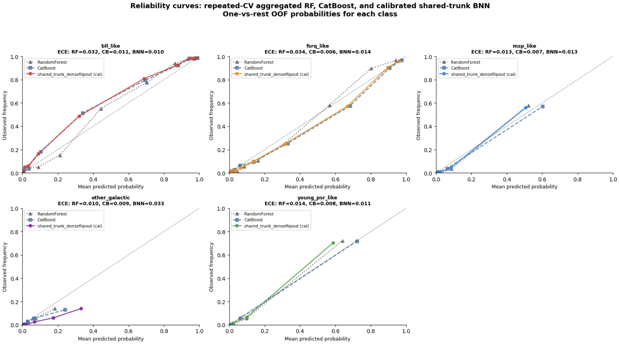
Across most classes, the new shared-trunk BNN tracks the ideal diagonal line very closely, meaning its predicted probabilities generally match reality quite well. In the blazar-like classes (bll_like and fsrq_like), all three models perform strongly, but the BNN and CatBoost tend to stay slightly closer to the diagonal at high probabilities. The young_psr_like class also looks noticeably improved for the BNN, with an ECE competitive with the other models. The one trouble spot remains other_galactic; all models continue to struggle there due to the tiny sample size and severe class diversity. Still, compared to the old BNN from previous weeks, these curves are a major step forward.
The next few plots we have capture the models’ uncertainty measures. Looking at the very left panel, we can see that the new BNN captures uncertainty much better than before. Compared to previous weeks, the uncertainty is more strictly and negatively correlated with the max probability. In other words, the new model is less uncertain for higher predicted probabilities, which is exactly what we want. Using the color-coding legend, we can also see that there are fewer incorrect predictions at higher probabilities than before.
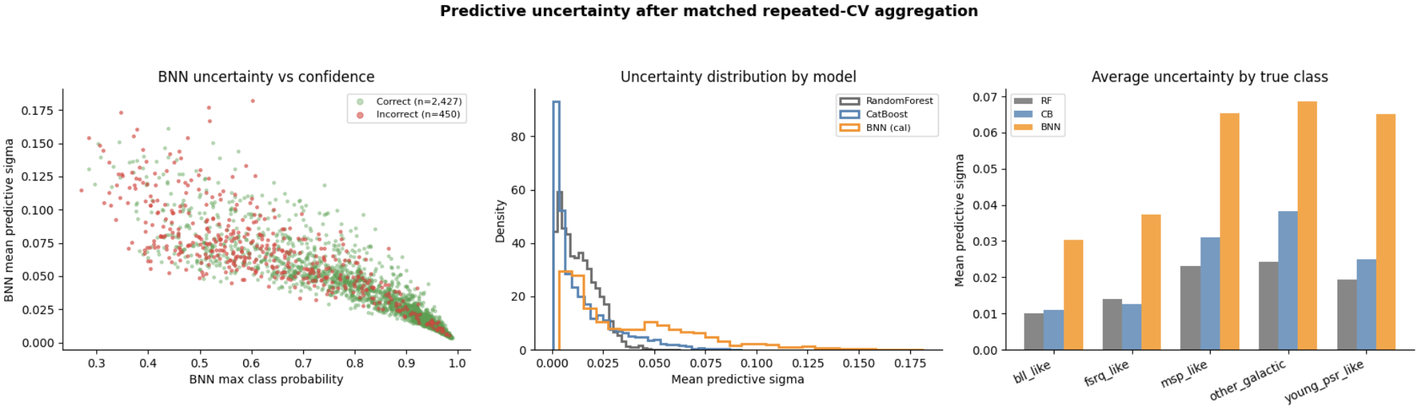
Now, let’s turn our attention towards the two plots on the right. Both plots compare the uncertainties of the three models. From the center plot, we can see that both baseline models’ uncertainties spike near zero, while the new BNN’s uncertainty is more spread out. The plot on the right confirms this, revealing that the BNN’s average uncertainty is higher across all classes. While this seems discouraging, it’s not completely unexpected or something to worry about too much. Since the baseline models don’t have uncertainty integrated into their model architectures, they only capture the variability between cross-validation repeats. On the other hand, the BNN incorporates the posterior predictive uncertainty as well. The BNN is therefore measuring something much broader, so a higher uncertainty doesn’t automatically mean it’s worse. That being said, it is definitely something we should look into next week!
Looking Ahead
Now that we’ve got more optimistic results, we can focus on refining and confirming the small details. In the table a couple of sections above, notice how I put the old-BNN numbers in red. I did that on purpose because those numbers aren’t entirely honest. That’s not to say they’re “wrong” in any way, but they just don’t tell us the full story. Unlike the other three models, the old BNN doesn’t use the correct prediction aggregation; it’s still using the old, overwritten-prediction scheme. For reliable comparisons, we should use the same aggregation strategy on the old BNN while keeping everything else the same.
Next week, I’ll focus on two things. The first will be to apply each change we discussed last week, one at a time, to the old BNN. This way, we’ll be able to see which changes create the most substantial improvements. Even though the new BNN performs quite well, it’s worth checking each fix to see if any of them are nonessential to the model’s enhancement. That would 1) give us a better idea of which architectural and training choices are actually driving the performance gains, and 2) possibly save us some computational complexity.
The second key area, which I mentioned when discussing the plots, will be to investigate the new BNN’s uncertainty. I have a couple of ideas in mind, which I’ll save for next week’s blog post. Stay tuned for the final week, where we’ll see how our ultimate model iteration performs. Until then, stay curious!
Acronyms
Here’s a list of all the acronyms used throughout this paper. I ordered them in terms of first appearance:
BNN – Bayesian neural network
CV – cross-validation
NLL – negative log-likelihood
ECE – expected calibration error
Leave a Reply
You must be logged in to post a comment.