Week 12: Messages from the Final Frontier
May 18, 2026
Hello, my fellow reader! It is with great joy that I welcome you to the final blog post of my senior project. I spent most of this past week tidying up my results for my paper and presentation. I’ve made a few small but important changes since I last spoke with you, so let me break them down and show you the closing results of this project!
John: One Fix At A Time
At the end of last week’s post, I mentioned that I would be seeing what happens if I applied changes to my model one at a time. Rather than running all of the changes to my original BNN at once, I’ve created two new iterations. The first only fixes the prediction aggregation, and the second includes all the minor improvements except the major architectural change. By splitting up the changes a little, I’ve been able to better understand which ones create the most improvement for my model.
Prediction Aggregation
With just the aggregation fix, my model’s evaluation metrics jump up significantly. This is as expected because, originally, the predictions were overwriting each other during training with every consecutive repeat. This made the repeated cross-validation process effectively equivalent to running only a single fold, which is not very robust for a model! Once all ten repeats are properly accumulated and averaged together, the model finally gets a much more stable and reliable estimate of its performance.
Architecture Comparison
Next, I’ve applied all of the changes I made last week, besides the architectural change. In other words, I’m using the three-model, hierarchical BNN, but incorporating all of the training and evaluation fixes we discussed last week. This essentially tells us whether the new, shared-trunk BNN architecture has any real benefit.
Now that we’ve applied the separate changes, we can compare their effects on our model in the table below. The first column shows the evaluation metrics for the original hierarchical BNN without any changes. The next column shows how performance changes when the predictions are aggregated, while keeping the same architecture. The third column then reflects the impact of all the other non-architectural modifications applied to the hierarchical BNN. Finally, the fourth column compares the shared-trunk hierarchical BNN with all of the changes that we made last week.
| OG BNN | OG BNN Aggregated Predictions | OG BNN All Other Changes | Shared-Trunk BNN | |
|---|---|---|---|---|
| Accuracy | 0.7810 | 0.8120 | 0.8186 | 0.8384 |
| F1 | 0.7762 | 0.8068 | 0.8071 | 0.8413 |
| ROC-AUC | 0.9328 | 0.9406 | 0.9502 | 0.9530 |
| NLL | 0.5450 | 0.5289 | 0.4882 | 0.4584 |
| Brier | 0.0570 | 0.0559 | 0.0515 | 0.0470 |
| ECE | 0.0285 | 0.0523 | 0.0412 | 0.0343 |
Looking at the table, we can see that the original BNN performs worst on nearly all of the metrics. Each new iteration makes small improvements over the last, which is exactly what we want to see. In the end, the shared-trunk BNN outperforms all three hierarchical variants, which tells us that: 1) the seemingly minor training and evaluation fixes we made actually did make a difference, and 2) the general learned representation of the shared-trunk BNN is superior to the isolated pathway approach of the hierarchical BNN.
Paul: Uncertain About Uncertainty?
Moving on to our next update, I’ve decomposed the shared-trunk BNN’s uncertainty. I’m doing this so that I can better compare the uncertainty to that of the baseline models. Because the tree-based baseline models are non-Bayesian, they don’t have that intrinsic uncertainty measure that comes from the posterior in Monte Carlo sampling. That means the BNN has an extra component of uncertainty, making the comparison unfair. So instead of using a single scalar to quantify the BNN’s uncertainty, I’ve split it up into two components.
Between-Repeat
The first is the between-repeat variance, which comes from how the data is randomly split for every cross-validation repeat. In every repeat, the model learns from a slightly different subset of training data, so there’s going to be some variation in its predictions. If we take the standard deviation of the predictions across all repeats, we can then derive an uncertainty quantification from this repeated cross-validation strategy. Since we use the same cross-validation scheme for the tree-based baselines, this uncertainty component is the one that’s actually comparable across all models.
Posterior Predictive
The second component is the built-in BNN uncertainty, which comes from the stochastic nature of the Bayesian heads in the shared-trunk hierarchical architecture. During inference time, the model is run 200 times with different weight samples drawn from its learned posterior, producing a distribution of predictions for each source. The variance across these MC draws captures how uncertain the BNN model’s own weights are, independent of how the data was split. This is unique to the BNN and has no equivalent in the tree-based models, which makes it harder to compare.
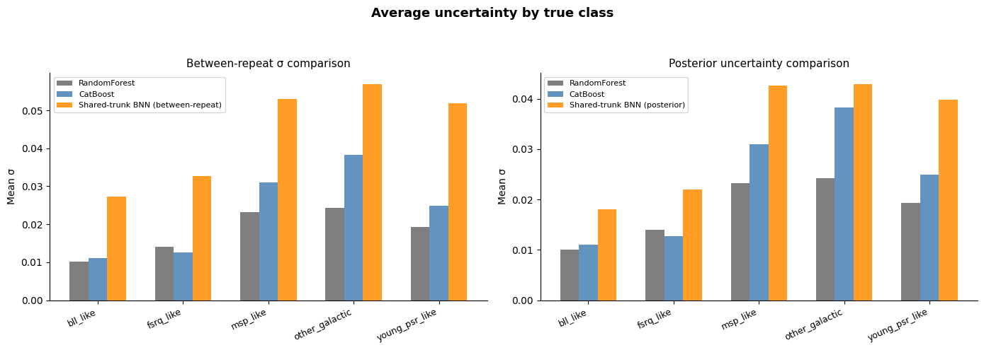
Now that we’ve split the uncertainty, we can more reliably compare it across the three models. In the first plot below, I’ve shown the average uncertainties for the different models. The left panel is the between-repeat variance that’s directly comparable across each model. We can immediately see that, even with the decomposed uncertainty, the BNN is still more honest. Both the Random Forest and CatBoost models underestimate their uncertainties. Interestingly, the posterior uncertainty tends to be slightly lower than the between-repeat uncertainty, but the two track each other pretty closely in terms of which classes the model is most uncertain about. All of the models seem relatively confident about the dominant bll_like and fsrq_like classes, but they remain more uncertain about smaller classes like msp_like and other_galactic.
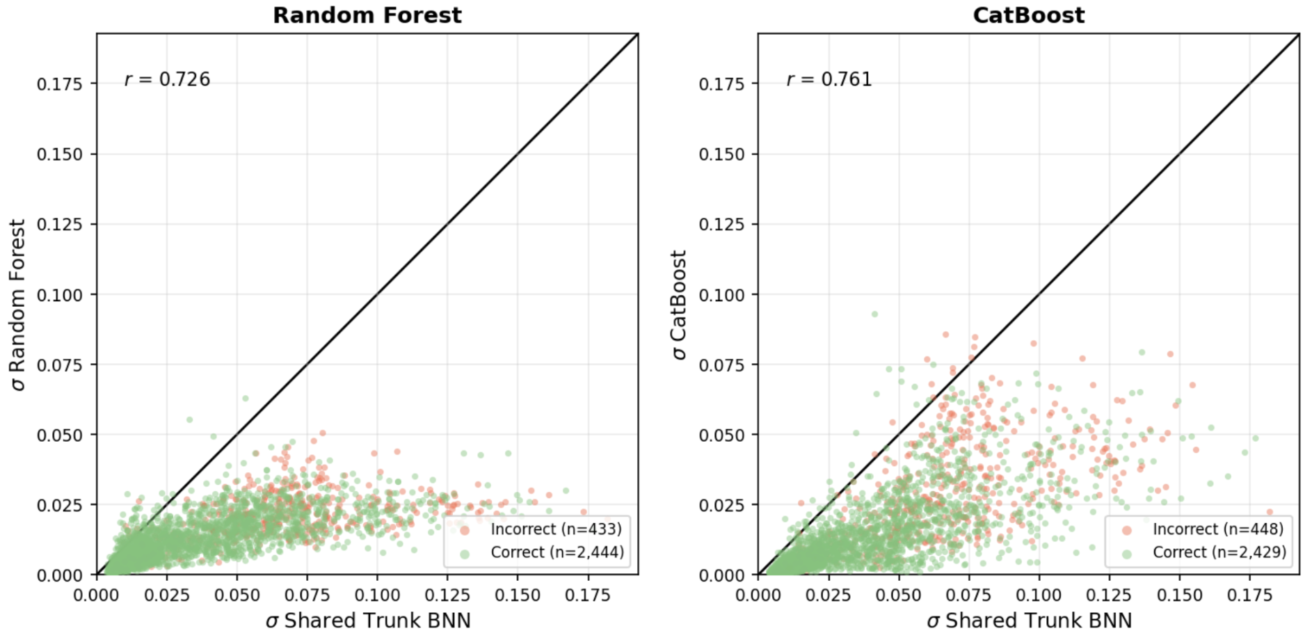
In this next plot, we can see the per-source uncertainties of each tree-based model plotted against those of the shared-trunk BNN. Essentially, it shows us the correlation between the baselines and the BNN. The uncertainty points for both the Random Forest and CatBoost models lie below the diagonal. This indicates that they’re overconfident in their predictions. Despite this, the correlations are reasonably strong, suggesting that all three models largely agree on which sources are hard to classify. The coloring of the points further reinforces this, as the incorrectly classified sources (shown in red) tend to sit higher and further to the right. This means that the higher BNN uncertainty is a reliable signal that a source is ambiguous. Overall, the BNN seems to report more uncertainty in the right places than the tree-based models.
George: Looking Ahead
If you’ve been along over these past twelve weeks, you’ll know that I always like to end every post with a short section that previews the following week’s tasks. Even though this is the last week of the senior projects, I still wanted to keep this practice. Except this time, it won’t be merely a look ahead into the coming week. Rather, it’ll be a discussion of the future work that could extend this research project.
Given the limited timeframe of this program, I didn’t get the chance to fully accomplish everything I had hoped for. Whether it’s taking completely new directions or making ongoing refinements to my model, there are a lot of ideas I have in mind that would take this project even further.
To improve my model, I’d like to experiment with various data augmentations. I’d first like to incorporate more data, whether that’s different types of data or data from different observatories. My project only used spectral and time variability data, but in the future, I’d definitely like to see how my model performs with additional types or instances of data. Along with that, I’d like to perform some data augmentation on my existing data. We could then see if that could account for the severe class imbalance. Previous papers have shown that this might not be the best solution[1], but you’ll never know until you try for yourself, right?
Once I’ve stabilized my BNN architecture, I’ll consider training more probabilistic models. I’m currently thinking about Gaussian Processes and Mixture Density Networks, but I’ll definitely look into more algorithms. This would be a good way to see how different probabilistic methods quantify uncertainty, and whether more complex architectures are better for this classification problem. The results of this study would be significant in helping researchers determine which probabilistic approach is best suited for classifying ambiguous gamma-ray sources.
Finally, but perhaps most importantly, I’d like to actually apply my model(s) to classify unassociated sources in the Fermi-LAT catalog. If you recall, the vast majority of sources in the Fermi-LAT 4FGL-DR4 catalog[2] remain unassociated. That was exactly what my project sought to tackle in the first place. Unfortunately, I didn’t get the time to accomplish that goal within these limited twelve weeks, but that simply leaves more exciting ground to cover in the future! Doing so would meaningfully advance our understanding of the high-energy gamma-ray sky, and potentially reveal new source populations in the process.
Ringo: Reflections
Before I bid you farewell for good (I know, I know, you’re getting tired of me), I wanted to take some time to reflect on this experience and to give my proper thanks to the people and resources that have supported me along the way. If you haven’t already noticed, the headings of each section in this post are the names of each Beatles member. This choice was inspired by that one scene in Project Hail Mary, where Dr. Grace sends his findings back to Earth using four space probes, each named after a different Beatle. Just like those probes carrying their discoveries across the void of space, each section of this post carries a piece of the work and thinking that went into this project over the past twelve weeks. It has been an incredible learning journey, with so many successes and challenges to reflect on.
These past several weeks have simultaneously felt like the longest and shortest period of my life. It felt short because I had so much fun devising, planning, and executing my project, but it also felt long because of all the requirements, deadlines, and lengthy blog posts. I’ve literally never written so much and so frequently in my life, but I am not complaining about that at all. In fact, I am so grateful to have had the opportunity to lean into my love for writing while documenting my project for you all to see.
Lesson Learned
Aside from the writing, I thoroughly enjoyed the continuous process of learning, succeeding, failing, and learning again. This project was in no way a linear climb, and I faced numerous challenges throughout. However, I think that might be the most valuable outcome of this project. Looking back on these twelve weeks, I’ve noticed both academic and personal growth. Whether it was searching (and asking Claude) to understand tedious equations or scrutinizing my code to find that one small error, every obstacle I pushed through made me a little bit better at this than I was before. I’ve definitely become a more knowledgeable and resilient researcher in the process.
For the juniors who are hopefully reading this, I advise you to pursue a passion project throughout your senior year. Even if you’re not asking for all of the structuredness and supervision of the senior project, you’ll gain so much from dedicating yourself to something you genuinely care about. In my very personal and non-biased opinion, I think the senior project is a great option. While it can be demanding at times, it’s an incredibly rewarding program that gives you dedicated time and resources to see a project through from start to finish. It’s a rare opportunity for you, a literal high schooler, to go out, meet professionals in your field, expand your network, and contribute to something you truly love. Plus, you’ll get to graduate with honors!
Acknowledgements
Yes, I’m very excited to graduate with honors, but I’m more proud of all the wonderful relationships I built with the people involved in this process. This project was so much less about the results and so much more about the people who made it memorable. It wouldn’t have been nearly possible without the support of so many brilliant and generous individuals. I’d like to take this time to thank each and every one of them.
First off, I’d like to thank my parents for always having my back and making the 2-hour round trip to SFSU every week. Without their benevolent Ubering services, I wouldn’t have been able to meet my external advisor, Dr. Oscar Macías, who has been an incredible mentor throughout this entire process. I’m so grateful that I was able to work with a professor who was so enthusiastic and knowledgeable, and always willing to point me in the right direction.
I’d also like to extend my thanks to my internal advisors, Mrs. Bhattacharya and Mr. Schindler, who were just as instrumental in getting me here. Between keeping me on track with deadlines, talking through technical difficulties, and offering emotional encouragement, their support was something I could not have done without. Of course, I’d like to acknowledge the school for providing the opportunity that made this project possible. And finally, I’d like to thank you, my dedicated reader, for bearing with me for this long.
With that, I’ll bid my final farewell. As TARS from Interstellar perfectly puts it, I’ll “see you on the other side.” It’s been an absolute pleasure, and until next time, don’t forget to look up!
Where To Find Me
If you were unable to make the final presentations, you can find the presentation recording linked below. Along with that, I’ve also provided the links to my presentation slides and GitHub repository. Feel free to check them out!
Presentation recording: https://drive.google.com/file/d/1e4NTtqUqvNhJtR-2jPlXgJjPDoU85rLP/view?usp=sharing
Presentation slides: https://canva.link/8x1hsvb62ehgut5
GitHub repository: https://github.com/chloelui/Fermi-Pulsar-BNN
References
[1] Butter et al. “Classification of Fermi-LAT blazars with Bayesian neural networks.” Journal of Cosmology and Astroparticle Physics, 2022. IOPscience, 10.1088/1475-7516/2022/04/023.
[2] NASA Fermi-LAT Collaboration. (2024). LAT 14-year Source Catalog (4FGL-DR4). Version 4, Fermi Science Support Center, 24 Jul. 2024, fermi.gsfc.nasa.gov/ssc/data/access/lat/14yr_catalog/. [Dataset].
[3] Boer, Poppe de. “The Beatles in Treslong.” Wikimedia Commons, 5 Jun. 1964, commons.wikimedia.org/wiki/File:The_Beatles_in_Treslong.jpg. Public Domain.
Leave a Reply
You must be logged in to post a comment.