Week 8 (4/13-4/17) - Clarifying the Pipeline With Text Prompts and the Initial Dive Into Interpretability

Welcome back to my blog! This week I finalized the text prompt formats for both datasets, dug deep into two important papers, and defined my pipeline even more, clarifying confusing steps in between. To start, I want to share what I learned from two papers I read this week on how incorporating interpretability would affect this project.

The first was a paper on retrieval-augmented generation, or RAG, in healthcare [1]. As I’ve mentioned in previous posts, I plan for RAG to be a core component of my pipeline, and this paper really explained why this is so important. The key idea is that RAG addresses gaps in a model’s knowledge by pulling in relevant external medical knowledge at inference time, then using that evidence to generate a response. The standard pipeline has three steps: indexing (external data is chunked and embedded into vectors for a database), retrieval (the user query is encoded and matched to the most relevant chunks), and generation (the model uses both the query and the retrieved evidence to produce an answer). One of the most compelling points is that RAG is more flexible and easier to update than fine-tuning when guidelines or practices change. However, it’s important to keep in mind that it can still inherit bias from its retrieved sources and may perform poorly for underrepresented groups if the source material is sparse.

The second paper I read was the original SHAP paper, “A Unified Approach to Interpreting Model Predictions” [2]. SHAP focuses on a single prediction and assigns each feature a contribution score for that specific instance, combining the same underlying additive feature attribution idea of most explanation methods. 

The features can be thought of like “players” in a game, where the payout is the model’s prediction. A positive value means the feature pushed the prediction up, a negative value means it pushed it down, and the magnitude tells you how strongly it mattered. This is built on three axioms: local accuracy (the explanation should exactly match the model’s prediction for the specific input being explained), missingness (a feature that is absent should get zero contribution), and consistency (if a feature becomes more important in the model, its attribution should not decrease). The paper also covers several variants, the most relevant being KernelSHAP, a model-agnostic method that explains any model by perturbing features and observing how the output changes. 

However, the paper raises an important caveat: the explanation still depends on how “missing” features affect predictions, which doesn’t directly apply to an LLM as words cannot literally be removed without replacement. This caution applies directly to my situation, since integrating SHAP with an LLM is significantly harder than with a model like logistic regression, where numerical feature contributions are straightforward to define. This is something I plan to consider carefully next week as I decide whether or not SHAP can still be integrated.

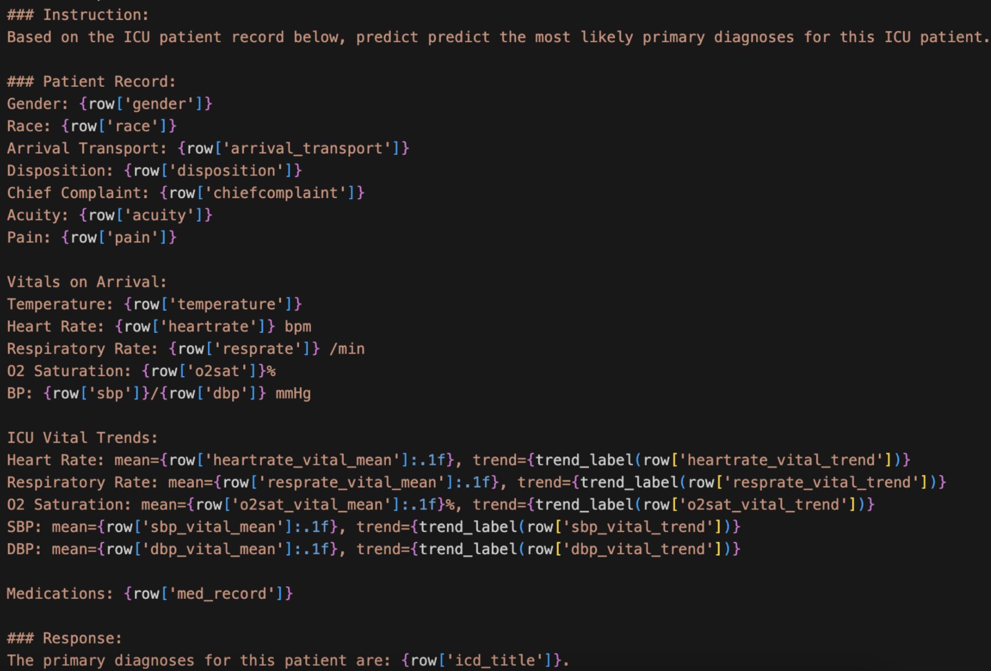
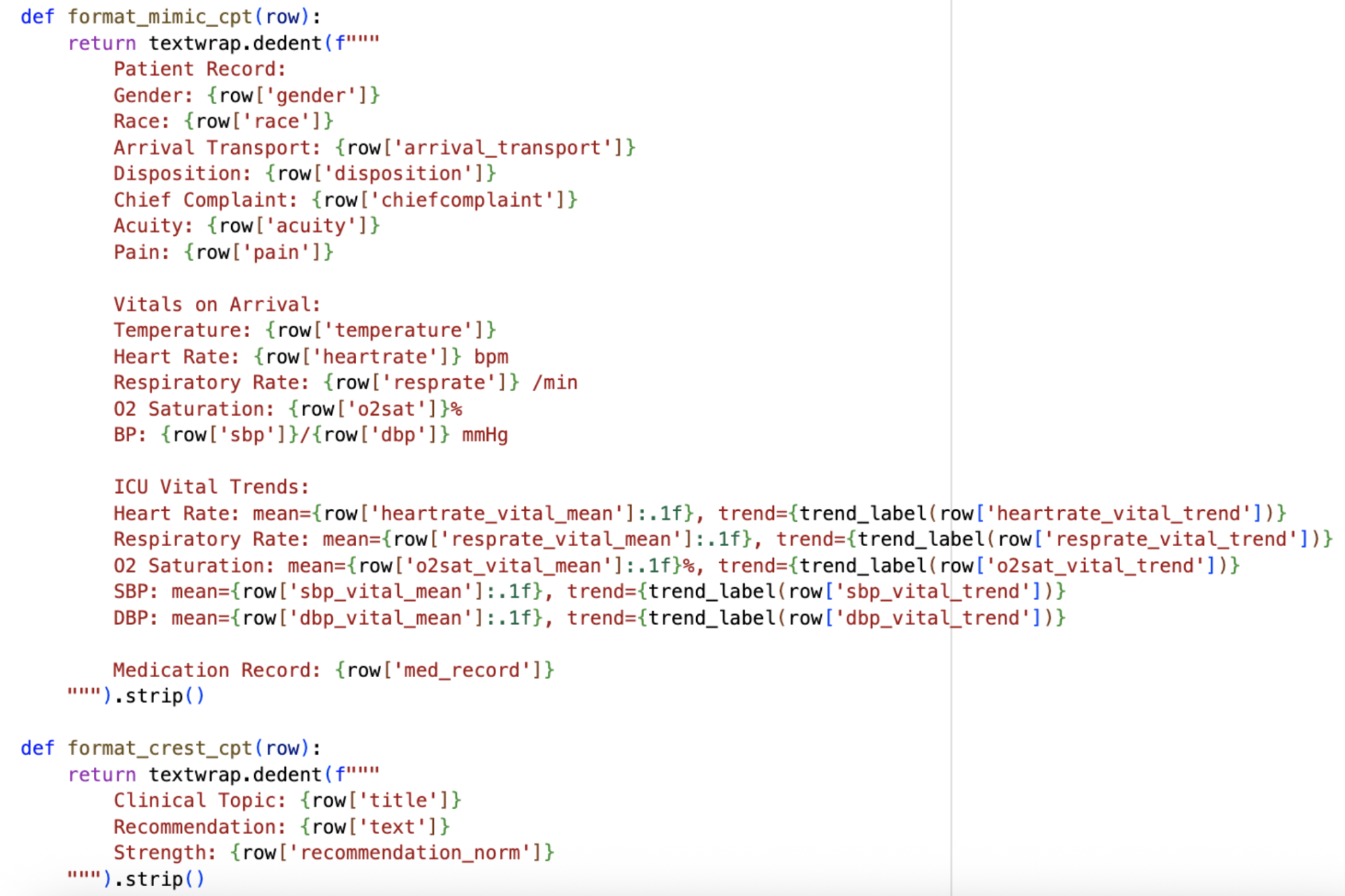
On the data preparation side, this week was all about converting both MIMIC-IV and CREST into text prompts for fine-tuning. For MIMIC-IV, I decided to separate the vitals from the information recorded at admission, since they represent different types of patient data. I also chose not to include medications administered during the visit for now, saving that for Stage 2 when CREST enters the picture, though the patient’s existing medical record is included. I also incorporated a trend label instead of just using the numerical value of the trend in the vitals. Since raw numbers for trends would be hard and confusing for a model to interpret, I created a label that simply classifies each vital as increasing, decreasing, or stable based on the values over time, making it much cleaner and easier for the model to understand.

For CREST, I similarly worked out a text prompt format to capture the key components from each guideline entry.

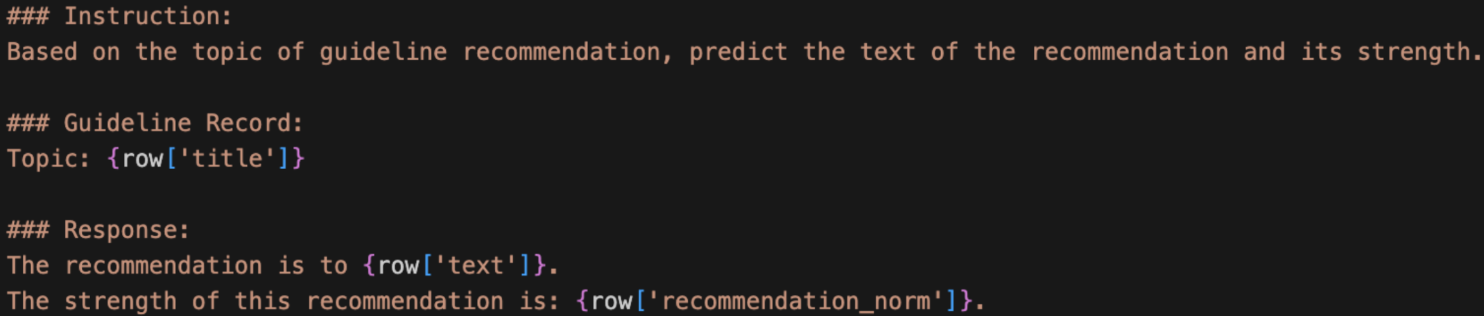
With both formats in place, I also updated my overall pipeline. I’m now redefining its phases: Phase 1 is continued pre-training (CPT) on raw MIMIC and CREST so that the model learns the medical domain. Phase 2 is instruction fine-tuning so that the model learns to predict ICD codes and generate recommendations, and it is in this phase I will incorporate RAG. With the given patient details, the model will predict the ICD diagnosis using the MIMIC text prompt above. Then, RAG will serve as the connection between MIMIC and CREST, matching the ICD of the predicted diagnosis to the CREST guideline topic using semantic similarity. Finally, the model would generate recommendations and corresponding strengths through the CREST text prompt, citing the retrieved guidelines with the developer of each recommendation. 

This new Phase 1 is based on the new topic I discovered this week, where I learned and explored continued pre-training (CPT). CPT exposes the model to domain knowledge before fine-tuning on any specific task. So, in my project, it would give BioMistral general familiarity with both datasets before it has to learn the actual prediction task. After thinking through how to connect MIMIC and CREST between all three phases, I landed on an approach for the CPT stage: simply shuffle both datasets together. The model doesn’t care about the order since it’s just absorbing information, and the shuffled format encourages the model to keep both domains (the datasets and their formats) in mind simultaneously.

There are potential benefits to CPT: an easier learning curve for fine-tuning (since medical abbreviations and patterns will already be familiar by the time task-specific training starts), slightly better handling of rare ICD codes that appear only a few times, and better generalization overall. Still, the downsides are also worth noting: it takes extra time and compute, and CPT is generally most useful when you have large amounts of unlabeled textual data, which BioMistral has already seen in its original pre-training. I’m not sure how useful CPT will be, which is why I am running it this week to see if the compute is feasible before committing to it.

For next week, the big goals are integrating RAG to connect the MIMIC and CREST phases of the pipeline, and investigating whether SHAP can still be incorporated in a meaningful way given the move to an LLM. The numerical contribution of each feature is much harder to define in this context compared to something like logistic regression, so this will require some creative thinking. Stay tuned!

[1] Yang, R., Ning, Y., Keppo, E., Liu, M., Hong, C., Bitterman, D. S., Chiat, J., Shu, D., & Liu, N. (2025). Retrieval-augmented generation for generative artificial intelligence in health care. Npj Health Systems, 2(1), 1–5. https://doi.org/10.1038/s44401-024-00004-1

[2] Lundberg, S. M., & Lee, S.-I. (2017). A Unified Approach to Interpreting Model Predictions. Semantic Scholar. https://www.semanticscholar.org/paper/A-Unified-Approach-to-Interpreting-Model-Lundberg-Lee/442e10a3c6640ded9408622005e3c2a8906ce4c2