Week 4: One Does Not Simply Estimate Differences (in Differences)

Last week, I began my data analysis after two weeks of collection and cleaning. The preliminary TWFE tests, which many economists have previously used as evidence of causality, revealed that the release of ChatGPT has increased the unemployment rate and hours worked, but not unemployment duration. However, the continuous differences-in-differences tests revealed no statistically significant relationship whatsoever. Given its stringent data requirements and low statistical power, I’ve sought alternatives that better satisfy relevant assumptions and provide higher statistical power. This week, I conducted analysis using discrete differences-in-differences and conducted pre-trend tests.

Discrete differences-in-differences

Discrete differences-in-differences is a lot like continuous differences-in-differences, except instead of continuous treatment exposure, there is a discrete one. To convert my continuous AI exposure indices and proxies into discrete groups, I binned them into quintiles. This means that every 20 percentiles of exposure will be grouped into one “binned” exposure. This has a few benefits and drawbacks. Given that I eventually do not find any statistically significant causal effects on hours worked and unemployment duration, I will pivot my focus to the unemployment rate, which is arguably the most important and relevant variable of interest.

You know what they say about Assumptions!

As discussed last week, continuous/multi-valued discrete DiD require the assumptions of parallel trends (PT) and strong parallel trends (SPT). I didn’t dive into the details of testing these assumptions because SPT is impossible to test, and PT could be visualized on the event-study plots. PT remained relatively unproblematic in continuous DiD, as zero remained within the confidence intervals prior to intervention. However, in multi-valued discrete DiD, due to its higher statistical power, PT becomes harder to satisfy as confidence intervals become smaller. 

Fortunately, SPT becomes more plausible in a discrete setting. Binning multiple exposure groups together produces a more stable estimate of the counterfactual trend, as it averages out noise across groups rather than relying on a single exposure group’s trend.

Checking for Parallel Trends

When analyzing pre-intervention trends, a visual inspection doesn’t reveal much. PT generally seems to hold across all bins at both the state-level and occupation level. Key note: I switched to occupation-level analysis to obtain a more varied measure of AI-exposure alongside more datapoints for multi-valued discrete DiD. After all, a balanced panel was no longer a data requirement.

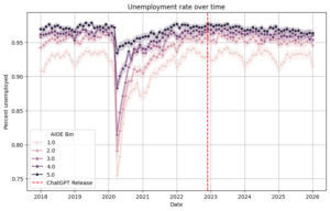
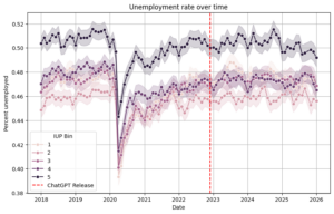
Using Callaway’s DiD package, including a function to check for PT, I compared every level of exposure to the lowest level of exposure, my primary counterfactual. At the state-level, without the need to control COVID-19, each exposure passed the PT test except for the second-lowest exposure. This should not be a significant issue, as later on, I will show that there was no statistically significant average treatment effect for the second-lowest exposure. At the occupation-level, even after controlling for COVID-19 by removing data from 2020, there were some issues. The highest and second-highest exposure bins did not pass the PT test. This could be problematic, as it may demonstrate self-selection effects with more AI-exposed occupations inherently following a different trend than non-AI-exposed occupations. There are additional methods to address these violations of PT tests, including a method introduced by Rambachan and Roth (2023) built in a package called HonestDiD. For now, I will continue my analysis with a nuanced causal interpretation of my occupation-level analysis.

With a Shaker’s Worth of Salt

Interpreting a multi-valued discrete DiD regression is very different from interpreting a TWFE or continuous DiD regression. Instead of a single value, we get 4; one for every exposure bin (except the lowest one), each measuring the average treatment effect (ATE) at that particular exposure.

At the state-level, the ATE monotonically decreases across each exposure level, with the fourth and fifth quintiles of exposure having statistically significant (p < 0.05) increases in unemployment. At the highest exposure level, ChatGPT increased unemployment by 0.81%. Similarly, at the occupation-level, the ATE shows an overall decrease in unemployment rate, with the fourth (p < 0.05) and fifth (p < 0.01) quintiles having statistically significant increases in unemployment. At the highest exposure level, ChatGPT increased unemployment by 1.32%. 

However, these estimates aren’t without their limitations. The AI-exposure index used for the state-level analysis was internet usage, an imperfect proxy for AI usage. Furthermore, the estimates only included 51 observations, as there was only one aggregated datapoint per group (in this case, fifty US states and one Washington DC). Similarly, the occupation-level analysis, though having more datapoints, did violate the PT test for the fourth and fifth quintiles, which were the only statistically significant quintiles. Thus, it is best to take these results with a grain of salt. Nevertheless, despite seeming worse than continuous DiD, these estimates have higher statistical power, more rigorous PT tests, and greater SPT validity.

The Practical and the Idealistic

At this point, I am starting to step into ethically grey areas. Am I really exploring different, similar methodologies to better satisfy assumptions and obtain higher statistical power, or am I really just trying to chase interesting results? Am I finding real relationships, or are these results driven by randomness, appearing due to the sheer number of statistical tests I am running? These are all questions that are very important to think about. I believe the answer to the first is that I am truly exploring methodologies. Though I wanted to explore unemployment duration, I dropped it when I didn’t find any interesting results. Similarly, I believe I can run discrete DiD without aggregation, increasing statistical power to ensure results are unlikely to be caused by spurious relationships. Nevertheless, I will continue asking these questions over and over again. In the following week, I will re-run multi-valued discrete DiD, test for parallel trends with the HonestDiD package, and reflect on the validity of my methodology.