Week 5 - Major Progress!
April 3, 2026
This week marked a major turning point in my project. I successfully resolved my prior issues with history counts, and generated my first graph!
Last week, I was running into a major issue with how TOPAS handled histories. Instead of producing dose data that was a function of x y and z positions, the program was only outputting a single summed dose value. This made it impossible to analyze how radiation was distributed across space. After troubleshooting (shoutout to Mr. Adams’ guidance!) I identified and fixed the issue related to how histories were defined in my main nano file.
Once corrected, I reran the simulation using millions of histories. This time, the output file, Dose.csv, increased dramatically in size, from just a few bytes to hundreds of kilobytes, and more importantly, now contained detailed rows of data corresponding to spatial coordinates (x, y, z) and dose values. This confirmed that the simulation was now recording dose as a function of position, rather than as a single aggregate value. Hooray!
With the proper data finally in hand, I moved on to visualization. I wrote a Python script (plot_heatmap.py) that processes the Dose.csv file and generates a 2D heatmap of the dose distribution. After running the script, I successfully produced my first image, which showed how radiation is deposited across the simulated region that included an organ and a tumor.
With this progress update, I’d like to briefly go through the process of how I went from setup to final image, involving many steps of debugging and implementation.
First, I identified the issue with histories by carefully reviewing my TOPAS setup file in nano. The problem stemmed from how the simulation was configured to record events, or “histories”. After correcting this, I ensured that the simulation was set to run with a sufficiently large number of histories and that scoring was properly defined across spatial bins.
Here is what my revised nano file looks like for my setup of choice — a section of a human chest — along with a brief breakdown of what each part means.
# ---------------------------------------------------------
# ICS HIGH-RESOLUTION K-EDGE SIMULATION
# ---------------------------------------------------------
i:Ts/NumberOfThreads = 0 # Uses all 10 threads detected on your machine
b:Ts/PauseBeforeQuit = "False"
b:Gr/Enable          = "False"
This section is the basic set up of my nano file, telling TOPAS to use all available threads to generate data (essentially increases the speed at which it could run histories), and also prevents the program from randomly pausing.
# PHYSICS
sv:Ph/Default/Modules = 1 "g4em-standard_opt4"
This section tells TOPAS which physics model to use. In this case, I used the Geant4 EM physics list optimized for low-energy electromagnetic interactions.
# 1. MATERIALS - MANUALLY DEFINED TO BYPASS DATABASE ERRORS
i:El/H/AtomicNumber = 1
d:El/H/AtomicMass   = 1.008 g/mole
s:El/H/Symbol       = "H"
i:El/O/AtomicNumber = 8
d:El/O/AtomicMass   = 15.999 g/mole
s:El/O/Symbol       = "O"
i:El/I/AtomicNumber = 53
d:El/I/AtomicMass   = 126.904 g/mole
s:El/I/Symbol       = "I"
This section covers the main elements used in my simulation — in this case, Hydrogen (H), Oxygen (O), and Iodine (I). Here, I have manually defined their atomic number, symbol, and also atomic mass to make sure TOPAS doesn’t run into errors or confuse itself.
# --- New Material: Bone (Calcium focused) ---
i:El/Ca/AtomicNumber = 20
d:El/Ca/AtomicMass   = 40.078 g/mole
s:El/Ca/Symbol       = "Ca"
Above, I have defined the primary material for my Bone setup, which will be mainly comprised of Calcium (Ca). Its atomic number, atomic mass, and symbol are all defined manually.
# Define the Dilute Solution directly from elements (5% Iodine, 95% Water)
sv:Ma/IodineSolution/Components = 3 "H" "O" "I"
uv:Ma/IodineSolution/Fractions  = 3 0.1055 0.8445 0.05
d:Ma/IodineSolution/Density     = 1.05 g/cm3
This section represents a solution of Iodine in water. Recall, I covered in previous posts that k-edge imaging requires a contrast agent that helps highlight the tumor when undergoing imaging. Iodine is a common contrast agent used in real-life medical imaging, and for my simulation, I will be utilizing a solution of 5% Iodine and 95% water. The solution’s element components, mol fractions, and density are included.
# Define a simple Lung (Water-equivalent density for geometry stability)
sv:Ma/MyLung/Components = 2 "H" "O"
uv:Ma/MyLung/Fractions  = 2 0.11 0.89
d:Ma/MyLung/Density     = 0.26 g/cm3
# Define a simple bone
sv:Ma/MyBone/Components = 3 "Ca" "O" "H"
uv:Ma/MyBone/Fractions  = 3 0.40 0.40 0.20
d:Ma/MyBone/Density     = 1.85 g/cm3
This section follows a similar format as the above, in which the compositions of my sample lung and sample bone are defined. It includes the elements in each material, their mole fractions, and also density.
# 2. GEOMETRY
d:Ge/World/HLX = 10. cm
d:Ge/World/HLY = 10. cm
d:Ge/World/HLZ = 10. cm
s:Ge/World/Material = "Air"
The Geometry section defines the shapes, sizes, and positions of objects I use. “World” as shown above refers to the total simulation space, which is filled with air.
# --- New Geometry: The Rib ---
s:Ge/Rib/Type     = "TsBox"
s:Ge/Rib/Parent   = "Lung"
s:Ge/Rib/Material = "MyBone"
d:Ge/Rib/HLX      = 0.2 cm
d:Ge/Rib/HLY      = 1.0 cm
d:Ge/Rib/HLZ      = 1.0 cm
d:Ge/Rib/TransX   = 1.5 cm  # Placed to the side of the vessel
These lines represent a setup of the ribs (basically a surface section of the chest).
# The Hook for the beam
s:Ge/BeamPositioner/Parent = "World"
s:Ge/BeamPositioner/Type   = "Group"
d:Ge/BeamPositioner/TransZ = -8. cm
This acts as a holder for the beam, ensuring it’s positioned correctly and precisely.
# The Phantom
s:Ge/Lung/Type     = "TsBox"
s:Ge/Lung/Parent   = "World"
s:Ge/Lung/Material = "MyLung"
d:Ge/Lung/HLX      = 5. cm
d:Ge/Lung/HLY      = 5. cm
d:Ge/Lung/HLZ      = 2. cm
This section represents the lung setup. This, along with the ribs setup above, completes a model for a portion of the human chest. Notice that these setups all contain the type of shape (box), where it’s located (world), the material (lung), and it’s precise coordinates (HLX HLY HLZ).
# The Vessel: Dilute Iodine Solution
s:Ge/Vessel/Type     = "TsCylinder"
s:Ge/Vessel/Parent   = "Lung"
s:Ge/Vessel/Material = "IodineSolution"
d:Ge/Vessel/RMax     = 0.1 cm
d:Ge/Vessel/HL       = 1.0 cm
s:Ge/Vessel/Color    = "Yellow"
This section is a simulated cylinder representing the iodine filled vessel (will be apparent on the simulation image).
# 3. MONOCHROMATIC ICS SOURCE
s:So/ICS/Type                     = "Beam"
s:So/ICS/Component                = "BeamPositioner"
s:So/ICS/BeamParticle             = "gamma"
d:So/ICS/BeamEnergy               = 30.0 keV     # Change to 30.0 keV for comparison run
s:So/ICS/BeamShape                = "Rectangle"
d:So/ICS/BeamWidthX               = 2. cm
d:So/ICS/BeamWidthY               = 2. cm
s:So/ICS/BeamPositionDistribution = "Flat"
s:So/ICS/BeamPositionCutoffShape  = "Rectangle"
d:So/ICS/BeamPositionCutoffX      = 2. cm
d:So/ICS/BeamPositionCutoffY      = 2. cm
s:So/ICS/BeamAngularDistribution  = "None"
i:So/ICS/NumberOfHistoriesInRun   = 1000000
This entire section defines the beam parameters. It shows beam details like size, energy, positioning, and also the number of histories I will run.
# 4. HIGH-RES SCORING
s:Sc/Dose/Quantity                  = "DoseToMedium"
s:Sc/Dose/Component                 = "Lung"
s:Sc/Dose/OutputType                = "csv"
i:Sc/Dose/XBins                     = 100
i:Sc/Dose/YBins                     = 100
i:Sc/Dose/ZBins                     = 1
s:Sc/Dose/IfOutputFileAlreadyExists = "Overwrite"
This final section is for scoring, which records the dosages received. It is “binned” (contained) in a 100x100x1 grid. Lastly, “Overwrite” means that if there is already an existing file, it will be replaced as you run the simulation again.
With the nano file ready, I could run the save command (control O + enter + control X). I was then able to run the TOPAS command using “topas TopasBone” (topas is the command to run the simulation, and TopasBone is the name I gave the file).
This step executes the full Monte Carlo simulation. The terminal output provides useful information, including the number of histories processed and confirmation that the scorer has written results to Dose.csv. I will cover below what that looks like.
Immediately after running, TOPAS will output a lot of the information about the setup, including copyright information for TOPAS, beam parameters, etc, and also effects like Coulomb scattering, which I won’t include here for sake of saving space.
Afterwards, TOPAS begins running histories. I will include a section below of what that looks like:
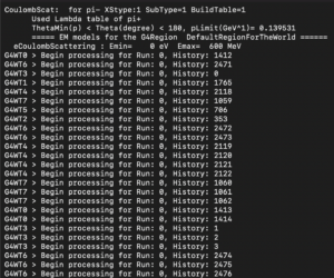
In this screenshot, you can see a small snippet of what the setup information looks like, and also how TOPAS runs histories. Remember earlier that I mentioned different “threads” that TOPAS will use — well, here it’s apparent why those are useful. These different threads help generate data in a parallel-processing manner, which greatly reduces the overall time taken. In fact, 1 million histories only takes roughly 10 seconds to run!
After all histories have run, TOPAS will output this final section before ending, in which it shows 1 million histories run, and that results have been sent to Dose.csv, a file for storing the data from the simulation run.
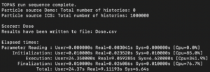
Apologies for the low image quality 🙁
Once the simulation completed successfully, I shifted to the Python portion. The purpose of this step is to transform raw numerical data in the Dose.csv file into a visual format that can be analyzed and interpreted. Using libraries such as Numpy, Pandas, and Matplotlib, the script reads in the CSV file, reshapes the data into a 2D grid (based on the binning defined in TOPAS), and displays it as a heatmap.
Below is what the python script looks like (plot_heatmap.py):
import pandas as pd
import numpy as np
import matplotlib.pyplot as plt
# —————————–
# Load the TOPAS Dose.csv file
# —————————–
data = pd.read_csv(‘Dose.csv’, comment=’#’, header=None)
# Get the last column (Dose) and reshape to 100×100
dose_map = data.iloc[:, -1].values.reshape((100, 100))
# —————————–
# Plot the heatmap
# —————————–
plt.figure(figsize=(8, 6))
plt.imshow(dose_map, origin=’lower’, cmap=’hot’, interpolation=’nearest’)
plt.colorbar(label=’Dose (Gy)’)
plt.title(‘TOPAS 100×100 Dose Heatmap’)
plt.xlabel(‘X bin’)
plt.ylabel(‘Y bin’)
plt.show()
Before running the Python script, I needed to set up a virtual environment. This ensures that all required libraries are installed and isolated from the system Python installation. I then activated the environment, and checked that terminal’s messages included a (myenv) in front, indicating successful activation. After installing the necessary packages, I executed the command “python3 plot_heatmap.py”, which ran my python script to generate a heatmap.
And finally, after 1444 words in this lengthy blog post, we reach the “punchline”:
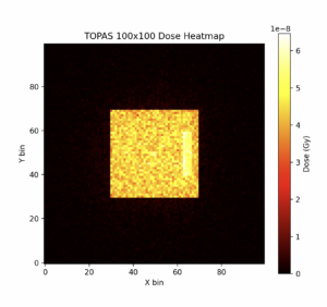
The above heatmap shows radiation dose on a 100×100 grid. The large yellow square represents the chest area that I tested on, and the small bright yellow rectangle on the right side is the tumor. This grid shows the radiation dose received by different parts of the area, and it’s evident that this ICS setup delivers a very strong dose to the tumor, and a much lower dose to the surrounding healthy tissue.
Looking ahead, I plan to focus on a few things.
First, I plan to test different simulation setups, including variations in geometry, materials, and beam energies, to better understand how these factors influence dose distribution.
I also aim to develop a different kind of graph, a line plot that shows dosage and highlights the K-edge effect.
And lastly, I will begin working on my final slides in preparation for the presentation in May.
More to come next week 🙂
Leave a Reply
You must be logged in to post a comment.