Week 10: Rewriting the Stars and My Model

Progress is never linear, and this week, I’ve really started to understand what that means. With only a couple of weeks left, you might want to assume that everything is slowing down and coming to an end. However, that’s not quite the case. We’re still going full steam ahead. This week, I’ve worked with my external advisor to devise new changes to improve the model’s evaluation metrics. Make sure to buckle up, because we’re in for a bumpy ride as we rewrite the model!

Room for Improvement

Last week, we saw small improvements in our Bayesian neural network (BNN) after making a small fix to the algorithm. While the BNN is heading in the right direction, it still performs worse than the uncalibrated baseline models. Ideally, we want to see the BNN performing at least as well as the two baselines, if not better. To this extent, there’s still some room for improvement. In the following sections, I’ll break down the major areas for improvement I’ll be working on over the coming weeks.

Break to Build

You’ve got to sacrifice something to gain something, right? Perhaps the biggest pivot this week is how we’re reconstructing the entire model architecture. Previously, we’d been working with a hierarchical model, where we would train three separate BNNs that each worked on a small classification task. The top-level BNN would identify galactic and extragalactic classes, while the two lower-level BNNs would distinguish specific object types within each class. While it seems like a logical approach, it’s extremely computationally expensive. Just think about how much extra time and space are needed to train three separate BNNs!

To subvert this problem, I’ve switched to using a single, shared-trunk hierarchical model. Let’s break this down a little. By “single,” I mean that we will only be training one BNN. If all goes to plan, that would save us from a lot of computational complexity. Moving on to the “shared-trunk” part, we’re essentially using one big, common trunk for the neural network that acts as the main feature extractor. It takes in all the data and input features to produce a shared internal representation of each source. Once the trunk’s gotten a general idea of the data, it splits into three separate branches. This is where the “hierarchical” part comes in. The three branches serve the same functions as the original three BNNs, but instead of being separate models, they’re now integrated as the final layers of a single network.

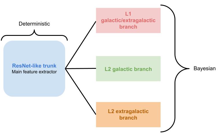
In this new model, only the final three branches are Bayesian. The main neural network body that does most of the feature extraction is a regular deterministic model with point-value weights. Prior research in tabular deep learning has shown that simple residual-network-like (ResNet) backbones are strong baselines for tabular problems^[1]. ResNets handle deep feature interactions well due to their skip connections, which is exactly what we need for our classification problem. Following these findings, we use a ResNet-like structure for the deterministic trunk. Only then do we attach the three Bayesian branches for fine-grain identification tasks. This further simplifies the model by introducing the Bayesian complexities only in the final layers.

No Data Is Data

Now that we’ve got the biggest change out of the way, we can move on to finer improvements. One problem I noticed is the missing entries in the second block of the feature matrix. This, which we called Block B last week, represents the high-energy spectral energy distribution (SED) measurements of each source. Last week, we simply used median imputation to fill in the missing entries, but didn’t actually expose the missing data. By doing this, we were losing valuable information because the fact that a value is missing carries its own significance.

In our new network, we create an additional layer of information to record the absence of data. We still keep the imputed median values so that our neural network learns properly, but we also add binary “missing” indicators to the network. This way, the model can learn possible patterns from missing data.

if transform.missing_cols.size == 0:
    missing = None
else:
    missing = np.isnan(x[:, transform.missing_cols]).astype(np.float32)

When In Doubt, Embed

This next fix is small, but it could benefit our model quite a lot. Previously, we’d been feeding all the numerical features directly into one dense layer. Essentially, all the standardized numerical values were stacked together into one long vector and fed to the first layer of the network. The network certainly got all of the data, but it also mixed everything all at once. This forced the first layer to understand what each feature meant and how features should interact. That can be a lot to ask on a first encounter!

The new iteration changes this by using feature-wise numerical embeddings. Before being combined with other features, each numerical feature is first given its own small learned representation. So instead of treating each feature as a single number, the model passes that one value through a tiny transformation to convert it into a short vector. This happens independently for each feature. For example, flux gets its own embedding, spectral curvature gets its own, each energy bin gets its own, and so on. Only after these individual embeddings are they concatenated and passed into the shared model trunk.

While this seems like an extra step, it lets the model learn each feature on its own before combining them. Some features have nonlinear importance, so feature-wise embeddings allow the model to capture that early. This way, the model can learn more meaningful information from preprocessed feature representations.

Aggregation Is Key

The final change I’ve introduced to the model relates to how we obtain the final prediction and uncertainty. This important fix could materially impact the evaluation metrics because they depend on the predictions and uncertainties.

At this point, I must admit that I made a mistake…but don’t we all? While looking back through last week’s code, I noticed that my model had been overwriting predictions on every fold. The setup used fifty global folds for repeated cross-validation so that each source could be held out and predicted multiple times across different repeats. However, the original model would take the latest prediction and overwrite the old one. This is incorrect because repeated cross-validation is specifically designed so that each source gets evaluated multiple times under slightly different training and validation splits. We’re losing a lot of information by throwing away older predictions.

The correct way to do this would be to average all of its repeated held-out predictions, not just the final one. Not only does this provide a more stable prediction, but it also handles uncertainty more accurately. The original model only captured the model uncertainty, but we also need the uncertainty across different repeats. Since each repeat trains on a different outer training set, predictions will also vary across each repeat. Our model needs to be able to capture this uncertainty as well, which is why we need this new fix. The new model uses the Law of Total Variance to explicitly combine both uncertainty sources.

Results

Unfortunately, I don’t have final results to present and make pretty plots with this week because I ran into an error. In the previous section, I talked about aggregating all the held-out predictions. However, since I didn’t use this method for the baseline models, there’s no way to compare the aggregated predictions. Visual Studio Code recognized that before me and angrily spit out this error message at me:

------------------------------------------------------------
ValueError                 Traceback (most recent call last)
Cell In[9], line 52
     39 rf_aligned, rf_proba, rf_std, rf_counts = 
     40 align_repeated_summary_to_train_df(
     41     train_df=train_df,
     42     agg_df=rf_oof,
     43     prob_cols=PROB_COLS,
     44     model_prefix="rf",
     45 )
     46 cb_aligned, cb_proba, cb_std, cb_counts = 
     47 align_repeated_summary_to_train_df(
     48     train_df=train_df,
     49     agg_df=cb_oof,
     50     prob_cols=PROB_COLS,
     51     model_prefix="cb",
     52 )
---> 53 validate_repeated_counts("RandomForest", rf_counts, 
     54 expected_counts)
     55 validate_repeated_counts("CatBoost", cb_counts, 
     56 expected_counts)
     57 print("=== Data status ===")

Cell In[8], line 148
    146 mismatch = np.where(observed != expected)[0]
    147 first = mismatch[:10]
---> 148 raise ValueError(
    149     f"{model_name}: repeated-CV validation counts disagree 
    150     for {len(mismatch)} sources. "
    151     f"First mismatches at rows {first.tolist()}: 
    152     observed={observed[first].tolist()} 
            expected={expected[first].tolist()}"
    153 )

ValueError: RandomForest: repeated-CV validation counts disagree 
for 2877 sources. 
First mismatches at rows [0, 1, 2, 3, 4, 5, 6, 7, 8, 9]: 
observed=[1, 1, 1, 1, 1, 1, 1, 1, 1, 1] 
expected=[10, 10, 10, 10, 10, 10, 10, 10, 10, 10]

I haven’t had the time to address this hiccup yet, but I assume that there’s a relatively straightforward fix. I’d probably have to apply the same aggregation pipeline to the baseline models and re-evaluate them. It definitely sounds a little tedious, but I want to aim for as much accuracy and integrity as possible here. I’ll continue working on it and report my results in next week’s post. Until then, stay curious, my fellow reader!

Acronyms

Here’s a list of all the acronyms used throughout this paper. I ordered them in terms of first appearance:

BNN – Bayesian neural network
SED – spectral energy distribution

References

[1] Gorishiniy et al. “Revisiting Deep Learning Models for Tabular Data.” Conference on Neural Information Processing Systems. 2021. arXiv, doi.org/10.48550/arXiv.2106.11959