Week 9: Hope on the Horizon
April 25, 2026
Hello, hello! Thanks for stopping by again! This week is special in more than one way. For one, I’m typing this out at an airport gate as I await my flight to China. The plane that will soar high into the sky and bring me there is a perfect metaphor for the progress I made this week. If you’ve been following along, you’ll know that the Bayesian models have experienced a few hiccups. But this week, things seem to be taking a turn for the better!
We Can Do Better
After discussing with my external advisor, I was able to pinpoint a couple of areas for improvement in my Bayesian neural network (BNN). The main problems I noticed were related to the input features and training loop choices. I’ll break down each tweak individually in the following subsections, so keep reading to find out!
Never Enough Data
If you recall, I’d created two subsections in my feature matrix. The first one, which we’ll call Block A, contains seven compact features from the Fermi Large Area Telescope (Fermi-LAT) catalog[1]. These features describe the overall properties of each source, such as its spectral shape and variability. The second one, which we’ll call Block B, consists of spectral energy distribution (SED) data. It shows the specific logarithmic flux values of each source across high-energy ranges.
Originally, I included only Block-A features for simplicity because they were the most comprehensive core features. This week, I’ve decided to include the Block-B features as well for a more detailed representation of the data. Here’s a list of both Block-A and Block-B features we’re feeding into our network this week:
| Block-A Features | Block-B Features |
|---|---|
| log10_Energy_Flux100 | flux_300_1000 |
| log10_Unc_Energy_Flux100 | unc_300_1000 |
| log10_Signif_Avg | flux_1_3 |
| LP_index1GeV | unc_1_3 |
| LP_beta | flux_3_10 |
| LP_SigCurv | unc_3_10 |
| log10_Variability_Index | flux_10_100 |
| unc_10_100 | |
| flux_100_1000 | |
| unc_100_1000 |
As you can see, the Block-B features are much more extensive. They provide a much better picture of the SED shape across energy ranges, but I didn’t include them initially because there are quite a few missing entries for these features. Nevertheless, they encode important information that could benefit our model. By using these features only when they are available, we can hopefully gain some extra points for our model.
Keep It Simple
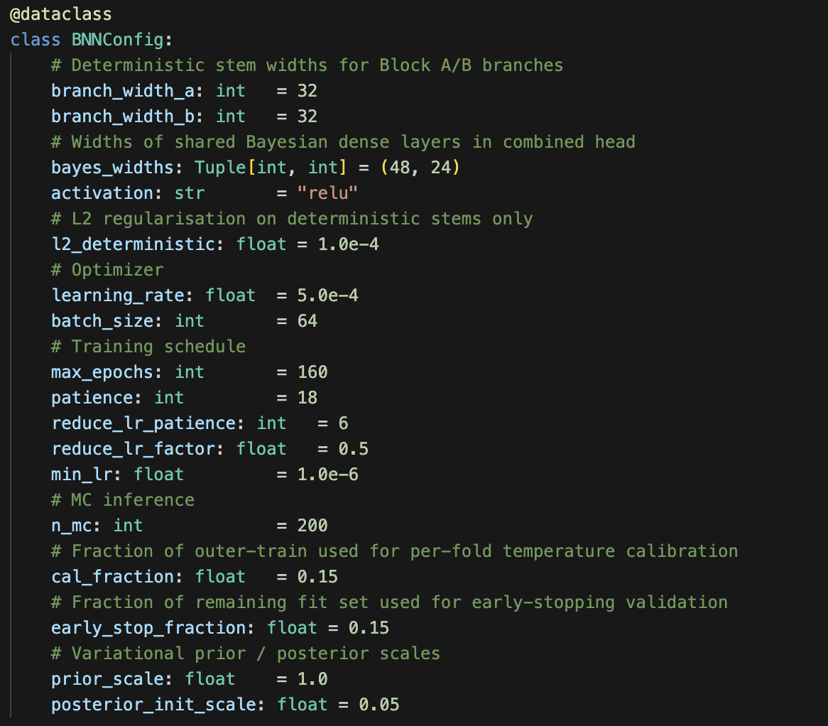
The next problem is related to the hyperparameters. Last week, I used Optuna to tune my hyperparameters. I basically used one of the cross-validation folds to tune the hyperparameters and applied those optimal values across all folds. While it seems like an efficient way to obtain optimal hyperparameters, it’s not very stable. Especially because I’m tackling three separate subproblems in my hierarchical BNN, I think it’d be better to stick with conservative default parameters. Once the repaired model is stable, I can consider adding back nested tuning. For now, let’s keep things simple.
A Little Remodeling
The final changes concern the model architecture itself. I’m making some small but important changes to how I structure the input data, compute the uncertainty, and fit the temperature scaling.
Data Normalization
In my original code, I added a BatchNormalization to the BNN input path. BatchNormalization is a popular data preprocessing step that normalizes input features across the batch dimension. It splits the data into multiple batches of samples. It then computes the mean and variance of each feature across all samples in that batch to normalize. The problem with this is that, given my relatively smaller dataset, the batches are small. With small tabular batches, training and inference behavior can become noisier.
Instead of normalizing across a batch of samples, we’re using per-sample LayerNormalization. Here, the normalization happens across the feature dimension for each sample independently. That means no more batch dependency, and no more batch dependency means that the behavior is the same at training and inference. This ensures that the normalization layer behaves consistently, making the entire process much more consistent.
Uncertainty
The next step is to fix how we calculate the predictive uncertainty. Last week, I made the mistake of combining the standard deviations for each of my three submodels in quadrature. I assumed that these standard deviations were independent and that they would propagate linearly into the final output. However, both of these assumptions are wrong. First of all, the uncertainties for the submodels are clearly related to each other because they depend on the same input. Second of all, the propagation is nonlinear. Let’s say we want to calculate the final probability for bll_like. We would get
P(bll_like)=P(extragalactic) x P(bll_like | extragalactic)
This is clearly a product of two random variables. Because we have a product of uncertain quantities, the final uncertainty is not simply the quadrature sum of the input uncertainties. The actual uncertainty in the product depends on both values and their joint distribution in a nonlinear way. It’s certainly more complex, but it’s a change we have to make if we want our model to improve.
To solve this problem, we’re computing the joint uncertainty through all three submodels. Rather than running each model’s passes separately and then combining the standard deviations, we simultaneously sample from the weight posteriors of all three at once. We get a complete set of weights that we can run through the full model hierarchy. This gives us a completely 5-class probability vector rather than a derived approximation.
Temperature Scaling
Last but not least, we’re changing how we perform temperature scaling. Last week, I fit the temperature on all out-of-fold (OOF) predictions. While that sounds reasonable, it creates a little bit of leakage. When we fit temperature on the pooled predictions, some of those very same predictions are the ones we’re later calling our “evaluation results.” This might make some of the evaluation metrics better than they’d actually be on new, unseen sources.
For a more accurate temperature fit, we’re giving temperature scaling its own dataset inside every fold. Essentially, we create a three-way split, where one chunk of data trains the model, one chunk finds the best temperature, and one chunk tests. Each fold also gets its own temperature instead of one global value shared across everything. The resulting metrics will hopefully be more reliable, as they’re genuinely measuring performance on data that was hidden from every part of the pipeline.
Did It Work?
So we’ve talked about all the fixes, but the real question is: do they actually improve our model? Thankfully, it seems like they do! The new BNN, with all of the aforementioned changes, has improved on many fronts. Just looking at the comparison table below, we can see that the repaired BNN has better values for all evaluation metrics. The accuracy, F1, and ROC-AUC are all higher, while the NLL, Brier score, and ECE are all lower.
| Accuracy | F1 | ROC-AUC | NLL | Brier | ECE | |
|---|---|---|---|---|---|---|
| CatBoost | 0.8394 | 0.8413 | 0.9455 | 0.4527 | 0.0460 | 0.0299 |
| BNN | 0.7588 | 0.7491 | 0.9193 | 0.6061 | 0.0662 | 0.0388 |
| Repaired BNN | 0.7810 | 0.7762 | 0.9328 | 0.5450 | 0.0570 | 0.0285 |
Although these improvements are small, they’re an optimistic step toward the right direction. We now have a better idea of what the model architecture might need more or less of. If we look at this next plot, we can see that the fix to the uncertainty calculation is a really significant choice.
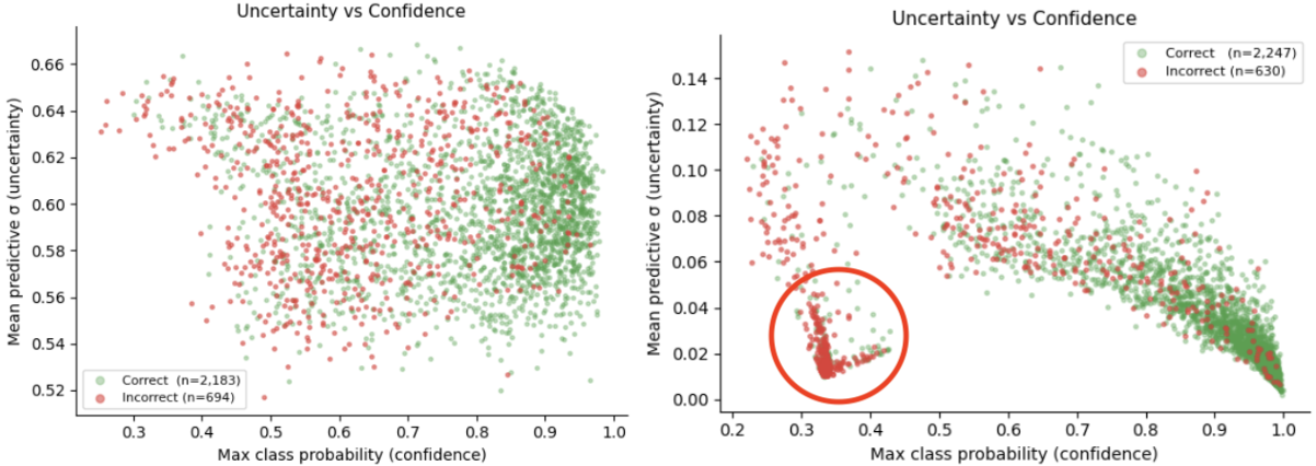
Immediately, we notice that the repaired BNN’s uncertainty (right panel) has a much more obvious negative correlation with confidence. In other words, the uncertainty of the repaired BNN is decreasing as prediction probabilities get higher, which is exactly what we want. The plots’ axes reveal another small detail. If you look at the y-axis of each plot, you’ll see that the maximum uncertainty value for the initial BNN (left panel) is 0.66, while that of the repaired BNN is only 0.14. So not only are the repaired BNN’s uncertainties less scattered, but they’re also smaller overall! That’s great news because it means our new computation method more accurately reflects the model’s uncertainty.
Looking Ahead
We certainly made some very meaningful progress this week, but it’s not all sunshines and rainbows yet. Looking back at the comparative uncertainty plots, you’ll notice something weird going on around the 0.3-0.4 probabilities for the repaired BNN. There seems to be an area of exceptionally small uncertainties, even for wrong predictions at low confidence. This is one of the missing pieces I’ll have to look into next week.
Along with this small caveat, I’m also planning to investigate the effects of additional small changes. For example, I might consider re-examining the imputation method for Block-B features or seeing whether nested hyperparameter tuning can be safely reintroduced. Since the current model relies on conservative defaults, there is likely still some performance left that could be revealed by a more robust tuning process. By refining how we handle these details, I hope to close the gap even further between our BNN and the CatBoost baseline. All in all, it’s been quite a productive week, and I can’t wait to see what the results look like once I’m back on solid ground. I’ll catch you all in the next update!
Acronyms
Here’s a list of all the acronyms used throughout this paper. I ordered them in terms of first appearance:
BNN – Bayesian neural network
Fermi-LAT – Fermi Large Area Telescope
SED – spectral energy distribution
OOF – out-of-fold
References
[1] NASA Fermi-LAT Collaboration. (2024). LAT 14-year Source Catalog (4FGL-DR4). Version 4, Fermi Science Support Center, 24 Jul. 2024, fermi.gsfc.nasa.gov/ssc/data/access/lat/14yr_catalog/. [Dataset].
Reader Interactions
Comments
Leave a Reply
You must be logged in to post a comment.
It’s really interesting how one adjustment can have such a huge effect on the overall results. I’m glad talking to your advisor helped you come up with a feasible solution. And writing a blog post from an airport gate is a commitment! Hope the trip goes well and looking forward to seeing what the next round of results looks like when you’re back.