Week 8: Segmenting the EDF Data for Results

Hi everyone, welcome back to my blog! Thank you everyone for all of the curious questions you’ve asked me, they’re really great and interesting questions that I’m looking forward to answering and discussing. This week was my heaviest workload yet, and I’m excited to share that we finally have significant results: I segmented the 24-hour data into 4-hour EDF data segments that can now be run in the pyHFO detection codebase, and I explored the classifications of each of the 150 4-hour EDF data segments into their specific Syngap1 mouse groups (heterozygous or wild-type with their treatments).

Over the past few weeks, after trying to run some manual detections on the original data which was talked about in last week’s blog, I created a script that I’m now using to handle this automatically. I split up the data into categories and used the EDF segmentation script we built last week to run all 150 of the 4-hour data chunks, summarizing each one’s HFO detections through the Markdown utility (which converts the .xlsx outputs into readable Markdown tables). The full run was planned to take over 12+ hours, and those outputs are now being analyzed for significant patterns, which I’ll dive into below.

To start off, I built a pipeline in the codebase so the resulting numbers are comparable across animals and conditions. From there, first, I applied the pyHFO segmentation script we built earlier, a single-purpose tool in which it opens an EDF, slices out a time window of 14400 seconds (4 hours), and then writes a new 4-hour EDF file. Then I set up a loop that reads each line of all the EDFs, creates the root between the files and pyHFO codebase, and applies the 4 hour segmentation script for every file. This roughly ran through all the EDFs and produced 150 segmented 4-hour EDFs in data_4hrs/ folder with 0 failures, taking up about 26 GB.

From there, across all of the 150 segmented 4-hour EDFs, we are now running detection with the pyHFO detection tool. For each EDF, it does three things: it filters the signal to focus on the HFO band frequency range (between 80 Hz and 500 Hz), it picks out possible specific types of HFO events using the STE algorithm (its algorithms which find short bursts of strong signal energy for spikes, the default detector pyHFO ships with), and then it sorts each candidate event into one of three categories using trained AI models on the GPU (artifact / spkHFO / eHFO), which we can then go into on the pyHFO application to accept whether that EEG signal is correctly represented as one of those categories. So through the Markdown utility, the pipeline would then also write two output files per 4-hour input: a *.4hr.npz file, which holds the raw event data (start and end times + the AI’s confidence scores), and a *.4hr.xlsx file, which is a readable two-tab spreadsheet for analysis where the Channels tab has per-channel summary counts and the Events tab has one row per detected event.

Before touching all 150 files, I initially ran into quite a number of issues surrounding the pyHFO detector needing specific editions of torch 2.8.0+cu128 (an ML framework) with open GPU compute so that it could run. After fixing those issues, I was finally able to start running the EDF files, but first I ran an initial test on one file (SynKI9-6(p60)_…_4hr.edf) end-to-end. It took 3 min 9 s, found 276 events, and wrote .xlsx and .npz cleanly. That gave us the per-file timing we needed to plan: 3 min × 150 ≈ 7.5 hours of GPU time. As I mentioned in earlier weeks’ blog posts about the use of the Markdown utility, the .xlsx file-type would now have this feature applied to the outputs of the detector. From there, I now created the batch setup, in which two parallel background loops were running: loop 1 detects all of the HFO events in the 4-hour segments, and loop 2 converts all of the data into the Markdown format, which scans and analyzes for different types of HFO events and their results.

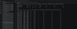
In the image above, it shows the finish of all 4-hour segments being run and detections being run through for all the files, and then we see the Markdown utility being applied to one of the many files that summarizes in tables the amount of different types of HFO detections and events across that specific 4-hour file. In that image, it shows the outputs of this 4-hour P60 EDF file, in which EEG_1_SA-B channel had 364 total detections (19 HFO, 6 spkHFO, 0 eHFO), EEG_2_SA-B channel had 242, EEG_3_SA-B channel had 336, and EMG had the highest at 427 total (414 HFO, 30 spkHFO).

Now that all of the 4-hour EDF files have been created with data and results for the total number of types of HFO detections, we are creating a script that will summarize our data into graphs and plots to compare all types of detections by age in specific channels such as EEG_2_SA-B, and the results should be promising if they show a progressive increase in all various types of HFO across the post-natal date increase, and then when treatment is applied.

So for next week, I will finally have some amazing plots to show, and we’ll compare across all the types of mice and figure out any issues that come up around detecting specific types of HFO like epileptic HFOs. We’ll see whether the number of HFO detections increases across the post-natal dates with all of the mice, including all types of genotypes such as wild-type with the treatment or heterozygous without the treatment. Next week, I look forward to showing and explaining the process of generating these plots and explaining their significance as biomarkers for Syngap1 mice!