Week 9: Collected data, differentiating spiders

Hello everyone, welcome back to another week of blog posts!

Given that most of the coding is already finished, I’ve published all my changes in code to the github repository. In addition, I’ve also updated the README file, which now contains a full guide in how to use my simulation, along with what’s needed to make adjustments (linked here).

Additionally, below are some data I’ve collected with the new model of ants that can fight back.

Data:

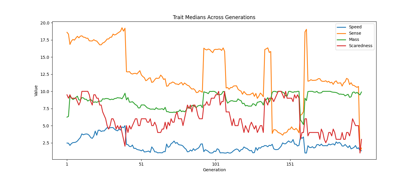
The first thing regarding data is that with ants fighting back, surivability becomes a lot harder. There are a lot of generations where no wolf spiders are able to survive, leading to the gene pool being completely reshuffled. The gene pool is sable only when a significant number of spiders who are good at surviving their niche all survive. For this reason, variance greatly decreased within traits of these spiders.

For this reason (and conciseness), I’m only going to show the median-over-time of all traits for these spiders. Just know that in every case the data surrounding the median are practically all direclty on the median.

For the same reason, I’ve also gotten rid of any genome that has survived for less than 30 generations. This gets rid of a lot of noise in the data, when an entire colony of spiders is wiped out and the simulation is back to randomly generating genomes. If you ever see any jumps between variables in the data, it means a previous surviving generation has died out and switched to a new generation.

Below is the first test I ran: wolf spiders against ants who fight back, vs ants who run away:

It can be a little hard to tell the difference between these two scenarios, so I’ve created some boxplots to represent the data.

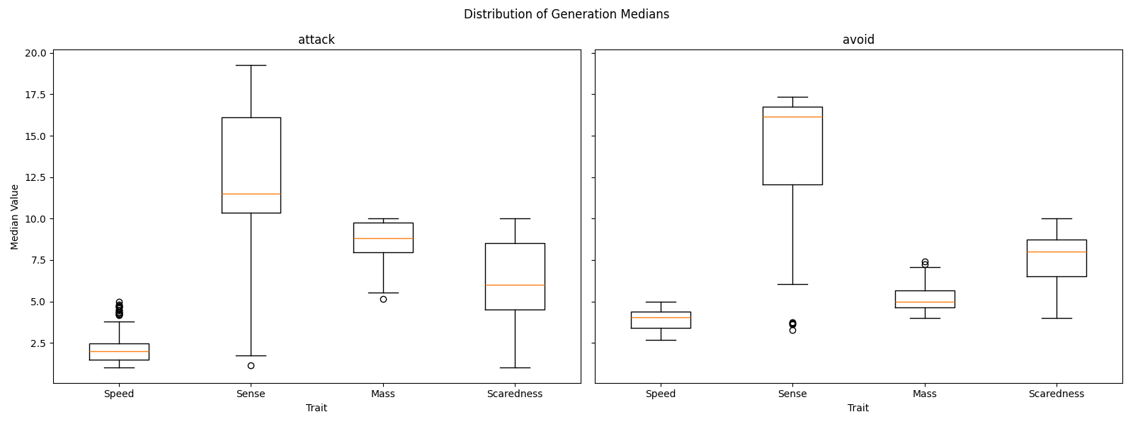
Using this plot, I concluded there was a statistically significant amount of difference in Mass and Speed, since the quartiles do not overlap. Keep in mind that sample sizes for both graphs were relatively big, so I found this result to be quite convincing that when spiders were up against aggressive ants, mass needed to be higher to reduce damage. Consequently, speed was lost as a trade off to keep the energy loss function abalanced.

For the second test, I compared wolf spiders in an environment where ants fight back, to the data I collected in previous simulations where the ants have yet to develop pheromones (blog 7). The results are as follows:

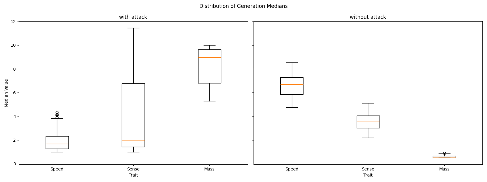
Both simulations were ran in an environment where ants were plentiful (60 ants). However, similar to the previous simulation of attack and avoid pheromones, in an environment with hostile ants, the wolf spiders were forced to significantly increase their “mass” state and sacrifice speed as a trade off, while having ants who don’t attack meant mass could be ignored entirely.

For the attacking simulation, sense was more important as well. Even though the wolf spider didn’t need high sense to find ants, having high sense could also help it avoid ant clusters, hence why the distribution on sense was so high.

Conclusions:

This concludes the data I’m collecting from the simualtions. In any case, I really enjoyed seeing how different spiders had to adopt different traits in order to stand against an ever changing environment. Seeing the “Mass” state gaining prominence, compared to the data in week 6, also made me realize how the traits all had their own importance as the simulation is built to be more and more complicated.

With the senior project coming to a close, I’m now turning my attention towards the icing on the cake. Hopefully, before I run out of time, I can update the models for ants and spiders from their current hand-drawn self by me.

It has been a very exciting journey so far working on this project. See you all next week, if I manage to get another blog out in time!