Week 5: Two Burns, Not Twenty
March 31, 2026
The agent has finally learned what it means to burn efficiently. Visit mazzola.dev for nicer formatting
01 — The Problem Left on the Table
Welcome back. Last week, the trained agent was reaching roughly the right altitude but was doing it wrong. Instead of two short impulsive burns (a prograde kick at perigee to elongate the orbit, a coast for roughly 20-30 steps, then a second kick at apogee to circularise), it was bleeding thrust continuously across the entire episode, ending with roughly the right orbit by sheer persistence.
The reward function was the culprit and two specific failures were embedded in its design. First, the SMA progress term rewarded the agent any time its orbit size increased, even past the target, so overshooting was costless. Second, the fuel penalty was calibrated as a “tiebreaker” rather than a real constraint, so the agent had almost no incentive to concentrate burns instead of spreading them out. This week I redesigned both.
| Source | Description | Focus |
|---|---|---|
| envs/env_config.py | Reward parameters: fuel_reward_scale, decisive_penalty, ta_bonus_scale, success_bonus, SMA potential redesign | Reward redesign |
| envs/hohmann_env.py | _compute_reward(): symmetric potential, doubly-quadratic ta_bonus, altitude-weighted eccentricity | Implementation |
| main_train.py | clip_range 0.2→0.1, ent_coef 0.005→0.015, net_arch [128,128], log_std_init=-1.0 | PPO tuning |
| tests/test_reward_shaping.py | 381 lines of unit tests verifying every reward component in isolation | New test module |
| Training runs v4, v6, v7 | 10M timesteps each across 12–14 parallel environments, randomised orbit distributions | Results |
02 — Redesigning the Reward
Reward shaping in reinforcement learning is a precise tool. Every term you add changes what the agent is maximising, and the changes interact with each other in non-obvious ways.
Change 1: Symmetric SMA Potential
The original progress term rewarded any increase in semi-major axis, regardless of whether the orbit was already larger than the target meaning that burning past the target was free. The fix is to replace the one-sided progress signal with a potential function that peaks at the target and falls off symmetrically in both directions:
# Before: one-sided, only rewards climbing
r_sma = (a_k - a_{k-1}) / (a_target - a_init) × 50

# After: symmetric, penalises both overshoot and undershoot
Φ(a) = -|a - a_target| / (a_target - a_init)
r_sma = [Φ(a_k) - Φ(a_{k-1})] × 50
# Moving toward the target is always rewarded, moving away is always penalised
This uses the potential-based reward shaping framework from Ng et al. (1999), which proves that any shaping reward of the form γΦ(s’) − Φ(s) leaves the optimal policy of the original task unchanged.
Change 2: Fuel Penalty Made Real
I raised the fuel penalty scale from 10 to 75. At the old scale, burning inefficiently cost almost nothing relative to the SMA progress reward. A wasteful agent that drained its tank over 40 steps accumulated a total fuel penalty of about -8.7 across the episode. A successful, efficient agent earned around +246. The penalty was barely visible. At 75x, the same inefficient tank-drain costs about -65, while an efficient Hohmann brings in roughly +172 total.
Change 3: Decisiveness Penalty
Even with a stronger fuel penalty, the agent could still satisfy it by consistently burning at a moderate fraction rather than oscillating between full burns and coasting. To explicitly push toward binary coast-or-burn decisions, I added a per-step penalty on intermediate burn fractions:
r_decisive = -0.5 × burn_frac × (1 - burn_frac)
# burn_frac = 0 (coasting): penalty = 0
# burn_frac = 1 (full burn): penalty = 0
# burn_frac = 0.5 (maximum ambiguity): penalty = -0.125
# Accumulates to at most -5 over a full 40-step episode
The shape of this function (x(1−x)) is zero at both extremes and peaks at the midpoint. Any burn that is neither a full commitment nor a coast gets penalised. The total per-episode penalty is small by design, because the goal is to tip the cost-benefit balance instead of dominating the signal.
Change 4: Location-Aware Burn Bonus
This is the most mechanically interesting change. A Hohmann transfer only works if burns happen at specific points in the orbit: burn 1 at the lowest point (periapsis) to raise the opposite side, burn 2 at the highest point (apogee) to circularise. The agent needed to be told that where you burn matters as much as how long you burn.
I added a per-step bonus that rewards burning near the right orbital location at each phase of the transfer. During the first half of the transfer (while the orbit is still small) the bonus rewards burning near periapsis. After the midpoint, it rewards burning near apogee. The bonus is zero at the wrong location and zero during coasting, so it does not punish coast arcs.
# Phase 1 (orbit smaller than midpoint SMA): reward periapsis burns
r_ta = 4.0 × burn_frac² × max(0, cos ν)²

# Phase 2 (orbit larger than midpoint SMA): reward apogee burns
r_ta = 4.0 × burn_frac² × max(0, -cos ν)²
# ν is the true anomaly (position angle in the orbit). cos ν ≈ +1 at periapsis, ≈ -1 at apogee.
Both the spatial term (cos²ν) and the burn-fraction term (burn_frac²) are squared, making this a doubly-quadratic profile. The spatial squaring concentrates the effective firing window to roughly ±70 degrees around the node: at 60 degrees off-node the bonus is only 25% of peak, and at 80 degrees it is 3%. The burn-fraction squaring is the subtler fix. With a linear-in-burn-fraction formula, there was always some positive marginal reward for starting any burn near the correct location, even a tiny one. The squared version makes the gradient zero at burn_frac = 0: no marginal reward for starting a small burn at all. Only committing to a large burn earns meaningful location bonus. This is what breaks the “small burns everywhere near apogee” local optimum that survived the first version of this term.
Change 5: Altitude-Weighted Eccentricity Shaping
Executing burn 1 sends the eccentricity from near zero (circular LEO) up to roughly 0.5 to 0.7 (the elongated transfer ellipse). Under the old reward, this spike was penalised immediately, even though it is a required step toward the final circular orbit. The fix ties the eccentricity shaping weight to how far along the transfer the spacecraft is. Near LEO the eccentricity term is weighted near zero. Near the target altitude the weight rises to full scale. Circularising in the right place earns a strong reward; the unavoidable eccentricity during the climb costs almost nothing.
Why the Changes Work Together: Each change closes one hole in the previous reward. The symmetric SMA potential stops overshooting from being free. The higher fuel penalty makes efficiency a real constraint. The decisiveness term closes the “moderate burns everywhere” loophole. The doubly-quadratic location bonus closes the “small burns near the right place” loophole. The altitude-weighted eccentricity stops burn 1 from looking worse than coasting. Together they leave exactly one local optimum: two concentrated burns at the right orbital locations.
03 — A Physics Problem: Why Not GEO
There was a second problem with the original setup that is not about reward design at all. The previous training target was GEO (geostationary orbit, roughly 42,000 km altitude). While this is a physically meaningful goal, it turned out to be impossible for the agent to reach within the 5% accuracy tolerance given the current thruster configuration.
The issue is gravity losses. When a thruster fires for an extended period, the spacecraft curves through its orbit rather than pointing straight in one direction. Part of the thrust goes toward fighting gravity rather than building orbital energy. The longer the burn relative to the orbital period, the more energy is lost. For a LEO-to-GEO transfer with a 1000 N thruster on a 750 kg spacecraft, reaching the transfer orbit apogee requires burning for roughly 50% of the orbital period. At that fraction, gravity losses eat about 18% of the theoretical energy gain. The actual apogee ends up at around 34,500 km instead of the required 42,164 km, an 18% error, far outside the 5% tolerance.
| Metric | Value |
|---|---|
| LEO orbital period consumed by burn 1 for GEO transfer | ~50% |
| Gravity loss on GEO transfer, 3.6× the 5% tolerance | 18% |
| Burn 1 duration for MEO (11,000 km) target, losses drop to 4.3% | ~16% |
The fix is to change the target to Medium Earth Orbit (MEO) in the 8,000 to 11,000 km altitude band. Burn 1 for this target spans only about 16% of the orbital period. Gravity losses drop to roughly 4.3%, which falls within the 5% SMA tolerance. The physics of the transfer are identical: same two-burn structure, same Hohmann geometry, but the shorter burn time makes the problem achievable without changing any equipment. GEO remains the long-term goal; it requires either a more powerful thruster or a finer time resolution (more decision steps per episode) to reduce each individual burn’s fraction of the orbital period.
04 — Steadying the Learner: PPO Tuning
Beyond the reward, I also changed several parameters of the PPO learning algorithm itself. These changes were motivated by observing what went wrong in the earlier runs.
Clip Range: 0.2 → 0.1
PPO’s defining feature is a clipping constraint that limits how much the policy can change in a single update step. The clip range parameter controls this limit. The standard default of 0.2 allows policy changes of up to 20% per update, which is appropriate for most continuous control problems. For this task, the doubly-quadratic reward landscape is unusually sensitive near the second burn: a small change in burn timing or location produces a large change in reward, which can translate into an oversized gradient update. Setting the clip range to 0.1 forces the policy to take smaller, more conservative steps. This alone had a measurable effect on training stability, particularly in avoiding the early collapse seen in the v6 run.
Entropy Coefficient: 0.005 → 0.015
PPO adds a small bonus for policy entropy, a measure of how “spread out” the agent’s action distribution is. High entropy means the agent is trying many different actions; low entropy means it has converged to a nearly deterministic strategy. In the v4 run the entropy eventually collapsed around 7.5 million steps: the policy became too confident in one particular (suboptimal) strategy, stopped exploring, and its performance cratered before slowly recovering. Raising the entropy coefficient from 0.005 to 0.015 keeps the agent exploring longer, preventing that collapse from happening so severely.
Network Width: 64×64 → 128×128
I widened both the actor and critic networks from 64 to 128 units per layer. The Hohmann task with randomised orbits presents 16 inputs and requires the agent to discover a phase-sensitive, two-burn strategy. The additional capacity gives the networks more room to represent the structured timing required.
Initial Action Distribution: log_std_init = -1.0
PPO for continuous actions represents the policy as a Gaussian distribution over each action dimension. The default initial standard deviation is 1.0, which produces a near-uniform spread across the full action range. Initialising with a smaller standard deviation (std ≈ 0.37) biases the agent toward more decisive actions from the start, reducing the amount of time spent in the noisy mid-range of the burn fraction during early training.
05 — Three Training Runs, Three Lessons
I ran three full training campaigns of 10 million timesteps each. The changes were introduced incrementally to isolate which factors were responsible for improvements and which introduced new instabilities.
| Run | Configuration | Best Result |
|---|---|---|
| v4 | clip=0.2, ent=0.005, ta_scale=2.0 | Best: 184 @ 9.8M steps |
| v6 | clip=0.2, ent=0.015, ta_scale=4.0 | Best: 191 @ 9.9M steps |
| v7 | clip=0.1, ent=0.015, ta_scale=4.0 | Best: 192 @ 8.4M steps |
v4: A Stable Run with a Bad Strategy
v4 introduced the full reward overhaul (symmetric SMA potential, higher fuel penalty, decisive_penalty, and an initial version of the location bonus at half scale) along with the wider 128×128 network. According to the training curve, the policy discovered a useful strategy around 1 million steps and held onto reward levels in the 175-183 range for the majority of training. The brief collapse around 7.5 million steps, followed by full recovery to 183 by 10 million, showed the policy converged too hard to one specific burn schedule, exploration collapsed, and it took another 1.5 million steps to shake loose.
Looking at the evaluation trajectories, v4 reaches the target orbit in every episode. However, we see the problem in the thruster command panel. Turns out, instead of a single decisive kick at apogee, v4 spreads its burn energy across the latter half of the episode with many small-to-medium burns.
v6: A Worse Collapse, a Better Recovery
v6 doubled the location bonus scale (from 2.0 to 4.0) and raised the entropy coefficient to 0.015 to address v4’s collapse, but kept the clip range at 0.2. However, rather than staying stable, the training collapsed even earlier, at around 1.5 million steps, and spent the next 6 million steps stuck near a reward of 33. This is far worse than v4’s brief late-run collapse.
A doubled location bonus creates steeper gradients near the optimal firing locations. With clip_range=0.2, a single gradient update could shift the policy enough to fall off the narrow reward peak and land in a flat, low-reward region. Once stuck there, the agent had to rediscover the correct strategy from scratch, which took 6 million steps. When v6 finally recovered around 7.5 million steps, it reached a higher peak (191) than v4 (184), confirming that the stronger location bonus is helpful once the policy finds the right territory.
v7: Controlled Steps, Cleaner Burns
v7 kept all of v6’s changes but reduced the clip range from 0.2 to 0.1. The smaller clip range forced the policy to take more conservative steps, preventing the large early collapse that plagued v6. The training curve shows a much healthier progression where the policy reaches useful performance around 1.5 million steps and improves steadily to a peak of 192.4 at 8.4 million steps. There is a brief instability around 6.5 million steps, but the recovery is fast. The run ends with a late-training collapse near 9.5 million steps that the training run did not fully recover from. The best model checkpoint from 8.4 million steps is what matters here.
At 192 reward, v7’s best model is the strongest result so far. More importantly, the shape of the trajectory has fundamentally changed.
06 — What the Trajectories Actually Look Like
The reward number is one thing. The trajectory is the real test. Here are the evaluation results from v4 and v7 side by side:
v4: Distributed Burns
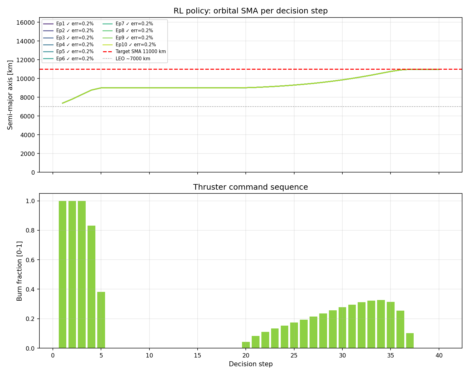
v4: all episodes reach the target, but the bottom panel shows burn energy spread across steps 15-40. No clear two-burn structure.
v7: Two-Burn Hohmann
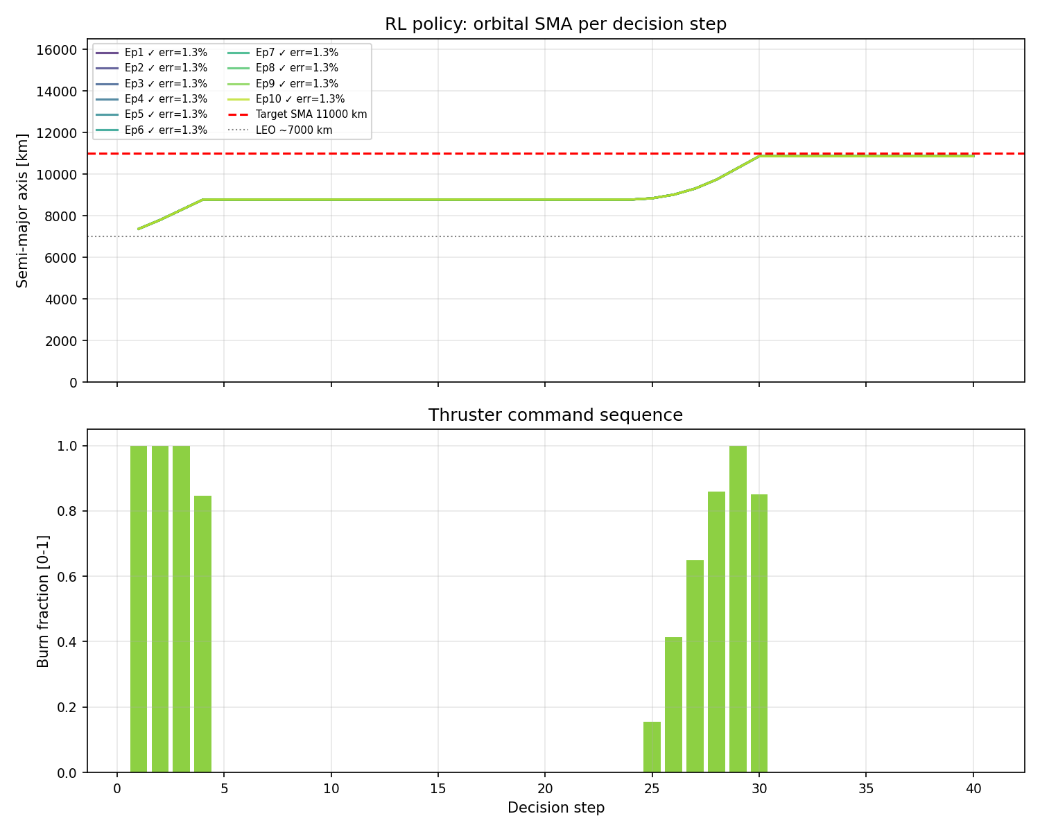
v7: burn 1 at steps 2-5 (periapsis), coast for 20 steps, burn 2 at steps 26-30 (apogee). All episodes land within 1.3% of the target SMA.
The bottom panel of the v7 plot showcases a concentrated burst of thrust at the start of the episode (when the spacecraft is near periapsis and prograde burns are most efficient), a long coast through the transfer ellipse, and then a second concentrated burst near the halfway point of the episode (when the spacecraft has reached apogee and a final prograde burn circularises the orbit). This is a Hohmann transfer, executed autonomously by a neural network.
The Oberth Effect in Practice: The reason burns at periapsis are more efficient than burns anywhere else in the orbit is the Oberth effect. It specifies that kinetic energy gained from a burn is proportional to F · v, where v is the spacecraft’s current speed. Orbital speed peaks at periapsis and is lowest at apogee. Burning at periapsis for burn 1, where speed is highest, delivers maximum energy to the orbit.
On Eccentricity Errors: The v7 trajectories show SMA errors around 1.3% and eccentricities of roughly 0.01 to 0.03, well within the tolerances of 5% and 0.10. The small residual eccentricity comes from the fact that the agent is making a finite-duration burn rather than an instantaneous kick. Burning across a range of orbital positions inevitably creates a slightly non-circular final orbit. Even the analytical oracle policy produces similar residuals for the same reason.
07 — What Comes Next
With a working Hohmann policy in hand, the next step is to stress-test this one. I’ll want to tackle the second part of my central research question for this project, which is whether a trained RL policy can handle uncertainties in real time. The plan is to make the model robust to perturbations by injecting noise directly into the observation and control channels during evaluation.
The long-term aim of the project is a policy that can autonomously correct for uncertainties in real time without ground intervention, which matters most for deep-space missions where communication delays make ground-loop corrections impossible. Testing the current Hohmann policy under perturbations is the first step toward understanding what that requires. If the policy collapses under moderate noise, that tells me something important about what the architecture or training curriculum needs to change before scaling to multi-gravity-assist scenarios.
There is also the late-training collapse in v7 to account for. The best checkpoint is from step 8.4 million, but the run ended in instability.
Next week: observation and control noise sweeps across the v7 best model and a diagnosis of where and how the policy breaks down under perturbation.
Reader Interactions
Comments
Leave a Reply
You must be logged in to post a comment.
Hi Nikola, seeing your agent work well must be extremely rewarding (no pun intended)! Figuring out and fine-tuning the reward function to be perfect is probably very difficult. Given the next steps to your research, do you expect that your policy can withstand noise in the system? How much noise do you expect it to handle, and how much does it realistically need to handle?
Hi Alex, you have perfect timing because I just wrote about this in my newest blog! The latest model was able to handle a significant amount of noise in the system. I aimed for 500 m position noise, 5% thruster magnitude uncertainty, 1 degree pointing error, unmodeled dynamics forces, and a 2% per-step chance of a burn failing. I worked my way up to these numbers, which is likely more noise than a spacecraft will face, but it builds robustness. However, I did learn that too much noise can hurt the policy because it ends up gaming the system by abandoning the clean two-burn behavior, so it’s important to get the balance right.