Week 7: Earth to Mars
April 21, 2026
Rebuilding the simulator around a moving planet, then running into a ceiling that tuning cannot fix. Visit mazzola.dev for nicer formatting
01 — Where We Left Off
Welcome back. Last week closed out the Earth-orbit problem by producing a robust two-burn Hohmann policy that held up under observation noise and thruster uncertainty. The research question for the rest of the project is whether the same can scale to a longer and more demanding transfer, so this week I rebuilt the simulator around an Earth-to-Mars trajectory and ran the first training campaign on the new environment.
The target policy is structurally similar with a Trans-Mars Injection burn at the right moment in Earth’s orbit, a coast arc of roughly 259 days, then a correction phase that steers the spacecraft toward Mars’s actual position at arrival. The implementation is almost entirely new as almost nothing from the Hohmann environment survived unchanged.
| Source | Description | Focus |
|---|---|---|
| envs/mars_transfer_env.py | New 952-line Gymnasium env: heliocentric frame, moving planets, two-phase episode, 18D observation | New environment |
| envs/env_config.py | InterplanetaryConfig dataclass: launch window geometry, departure/arrival planet parameters, phase step budgets | New config |
| utils/bsk_utils.py | build_interplanetary_simulation(): Sun-centred sim with Earth + Mars as gravity bodies driven by writable state messages | BSK builder |
| main_train.py, main_validate.py, main_montecarlo.py | Unified behind an –env flag so the Earth and Mars envs share the same training, evaluation, and MC pipeline | Shared scripts |
| tests/test_mars_env.py | 35 new tests covering the Gymnasium contract, heliocentric physics, reward components, and full-episode survival | New test module |
| runs/mars_v2, mars_v3, mars_v5, mars_v11 | Four training campaigns diagnosing departure-burn incentive design; v11 is the first converged model (~335 reward, 100% arrival) | Results |
02 — A Different Gravity Problem
In the Hohmann env, Earth was front and center. The spacecraft orbited a single point mass and every position was measured from Earth’s center. For an interplanetary transfer that frame is wrong. The spacecraft is in a parking orbit around Earth, but Earth itself is orbiting the Sun at 29.78 km/s, which is roughly four times the spacecraft’s orbital speed around Earth. Ignoring that motion and placing Earth at a fixed point produces a simulation that is inconsistent with itself the moment the spacecraft leaves low orbit.
The new simulator uses a Sun-centred inertial frame. The Sun sits at the origin with the Earth and Mars modelled as gravity bodies orbiting it on circular paths. Basilisk exposes each planet’s state through a SpicePlanetStateMsg, which is normally populated by a SPICE ephemeris file but can also be written directly. I take the second approach: at every simulation sub-step the environment computes each planet’s position and velocity from its circular-orbit parameters and writes them into the message.
# Circular-orbit planet state at simulation time t
θ(t) = θ₀ + ωt,   ω = v_helio / r_helio
r_planet(t) = r_helio [cos θ, sin θ, 0]
v_planet(t) = v_helio [−sin θ, cos θ, 0]
Refreshing planet positions at every sub-step rather than once per decision step matters during the departure phase. Earth moves about 8.9 million metres in a single 300-second decision step while the parking-orbit radius is 7 million metres, so a stale Earth position would warp the LEO dynamics by more than the radius of the orbit itself, so the planet-state write happens inside every 10-second burn sub-step and at every coast-chunk boundary.
The 104-Day Clock
Basilisk tracks simulation time as an int64 count of nanoseconds, which overflows at roughly 2⁶³ / 10⁹ ≈ 9.2 × 10⁹ seconds. That is more than two centuries in real time, but the internal API for time conversion uses a smaller accumulator that overflows at around 104 days. A full Earth-to-Mars episode needs roughly 337 days of simulated time (the 259-day Hohmann coast plus margin for the agent to arrive late), which is more than three times that limit.
The fix is to chunk the coast phases into segments no longer than 85 days each. At the end of each chunk the environment pulls the current spacecraft position and velocity out of the simulator, tears the Basilisk simulation down, and rebuilds it from the saved state with the time accumulator reset to zero. This is invisible to the RL agent as the observation it receives the moment before the rebuild and the one it receives the moment after are identical.
The Launch Window
In a real Hohmann-type transfer to Mars, the departure moment is chosen so that Mars will be at the spacecraft’s aphelion when the spacecraft arrives there. The geometric condition is:
θ_Mars(0) = θ_Earth(0) + π − ω_Mars × T_Hohmann
# Mars has to "lag" by exactly the angle it will sweep during transit
With T_Hohmann ≈ 259 days and Mars’s orbital rate of about 0.524°/day, Mars starts the episode roughly 44° ahead of Earth in its orbit, and by the time the spacecraft has traced half an ellipse around the Sun, Mars will have swept forward to the meeting point. Every episode resets to this ideal geometry, which keeps the problem clean for first-run training.
03 — Two Phases at Two Scales
The biggest challenge is the scale mismatch between the departure burn and the coast arc. The Trans-Mars Injection burn is a few minutes long and has to hit a precise point in a 90-minute LEO orbit. The coast lasts nine months. Using a single time resolution for both wastes computation if it is fine enough for the departure, and makes the departure unsolvable if it is coarse enough for the coast.
The episode is split into two phases with independent step durations. Phase 0 covers Earth departure at Δt = 300 s, giving 40 decision steps across roughly 3.3 hours. Phase 1 covers heliocentric transit and Mars approach at Δt ≈ 3.4 days, giving 100 decision steps across the full 336-day transfer. The agent sees a single continuous episode of 140 steps and a single 18-dimensional observation vector; only the internal integrator timescale changes.
| Parameter | Value |
|---|---|
| Phase 0 decision step (LEO departure) | 300 s |
| Phase 1 decision step (heliocentric transit) | 3.4 d |
| Total decision steps per episode | 140 |
Departure: Geocentric Prograde
Phase 0 burns apply thrust along the spacecraft’s velocity relative to Earth, using the geocentric frame instead of the heliocentric one. This is the direction that makes the Oberth effect work during escape from Earth’s gravity well. The thruster force is raised to 4 kN (the Earth-orbit env used 1 kN) so that a full-duration Phase 0 burn delivers up to 1440 m/s of Δv. The theoretical TMI requirement is roughly 3526 m/s, so 2 to 3 aligned full burns suffice, which fits comfortably inside a single LEO orbit pass.
A lower thrust setting is actually worse for this problem. At 2 kN, the same burn magnitude needs 5 or more steps, and each burn stretches the orbit slightly so the next periapsis arrives later in the episode than the previous one. The agent never sees the same periapsis twice, making it hard to learn the timing pattern. At 4 kN all the necessary Δv can be delivered inside one periapsis window, so the agent only has to learn the single correct moment to fire.
The Alignment Observation: The observation vector includes a scalar tmi_align term, defined as max(0, v̂_geo · v̂_Earth). It is 1 when the spacecraft’s geocentric velocity points directly along Earth’s heliocentric velocity (the Oberth-optimal moment) and 0 when they are perpendicular or anti-parallel. This tells the agent directly how aligned the current moment is for an escape burn, without having to infer it from the raw position and velocity vectors. Every tested training run that omitted this term failed to discover the correct timing within 10 million steps.
Transit: Cross-Track Corrections
Once the spacecraft has escaped Earth’s sphere of influence, the dynamics flip. The Sun becomes the primary gravitational body, Earth becomes a point moving away in the background, and the agent’s remaining job is to steer toward Mars’s arrival position. Burns here are small (capped at 14.5 s per step for roughly 89 m/s) and are applied in the cross-track direction: the component of the spacecraft-to-Mars vector perpendicular to the current heliocentric velocity.
Cross-track was chosen over a “burn toward Mars” heuristic because Mars is roughly 9° ahead of the spacecraft’s velocity vector at arrival. A burn pointed at Mars would put 99% of its Δv along the velocity direction, adding orbital energy and pushing the aphelion past Mars. The cross-track projection rotates the orbit’s orientation while leaving its energy untouched, which in principle lets the agent correct for departure direction errors without overshooting. I will come back to this choice in the last section.
04 — Reward Design for a 140-Step Episode
The Hohmann reward recipe from last month does not transfer directly. The agent has to solve two different sub-problems, and the signals that worked for a 40-step episode fire too sparsely to drive learning across a 140-step one. The Mars reward has four shaping terms plus a terminal component.
Alignment-Weighted Departure Bonus
Phase 0 needs its own positive signal because the distance-to-Mars shaping is essentially flat while the spacecraft is still inside Earth’s sphere of influence. The bonus rewards mass burned during departure, weighted by alignment:
r_depart = (Δm / m₀) × (base + scale × tmi_align²) + r_fuel
# With base = 0, scale = 200, fuel_scale = 50:
# Net per burn = Δm/m₀ × (200 × align² − 50)
# Breakeven at align ≈ sqrt(50/200) = 0.50
The first three Mars training runs (v2, v3, v5) all failed at this term. v2 had no departure bonus and the agent simply coasted for every episode. v3 added a flat per-burn bonus and the agent burned at every step regardless of alignment, wasting fuel on retrograde kicks. v5 used a bonus that scaled linearly with alignment, which was still net-positive at alignments below 0.5 and produced the same unselective behaviour. v11 uses the quadratic alignment weight with a base of zero, which gives the agent the choice where burns at alignment below 0.50 cost more fuel than they earn, burns above 0.50 are profitable, and the optimal moment (alignment near 1.0) dominates everything else.
Why Random Initial Exploration Still Works: A breakeven at alignment 0.50 raises the question of whether random Phase 0 burns produce enough positive samples to bootstrap learning. Roughly half of Phase 0 timesteps have the spacecraft in the prograde half of its LEO orbit, so about 50% of random burns land above breakeven. That is enough for the value function to notice a correlation between high alignment and positive reward within the first 100,000 steps, which is what v11’s training curve shows.
Distance-to-Mars Potential
The heliocentric shaping term is a potential-based function on the distance to Mars, normalised by the initial distance. It follows the Ng et al. (1999) framework from Week 5, which keeps the optimal policy unchanged while supplying a dense gradient. Closing the gap earns positive reward at every step, widening it costs the same reward, and the per-step magnitude is small enough not to overwhelm the departure bonus during Phase 0.
Graded Terminal Bonus
A 20 million kilometre success threshold (0.134 AU, chosen from the oracle’s empirical 7-10 Mkm achievable closest approach) is reached in most episodes once the agent learns departure. For the episodes that fall outside the sphere, a graded bonus fills in the missing gradient:
r_prox = 100 × max(0, 1 − d_min / (2 × d_success))
# d_min: closest approach to Mars achieved during episode
# Active inside 40 Mkm, zero beyond
An episode that closes to 25 Mkm (just outside the success sphere) earns a proximity bonus of roughly 38, while one that closes to 50 Mkm earns zero. The success bonus itself is 200, so an actual arrival is still preferred over any proximity outcome by a wide margin. The purpose is to provide a distinguishable reward signal between “close miss” and “way off”, which turns out to be the difference between the agent learning anything at all in Phase 1 and flatlining.
No Fuel-Depletion Termination
One of the subtler changes is that running out of fuel does not end the episode. With 4 kN thrust and the action range [0, 1], a random policy empties the tank within 7 steps, and earlier versions of the env then truncated the episode with a failure penalty. The problem is that this cuts off the agent’s exposure to Phase 1 entirely before it has learned to be selective in Phase 0, so the distance-to-Mars gradient never reaches the policy. Now an empty tank simply means every subsequent burn command is silently ignored while the episode continues to run. The agent still coasts for all 336 days and receives the distance-based rewards, including the proximity grade, based on whatever trajectory it ended up on.
05 — mars_v11: First Converged Model
v11 trained for 10 million steps on 8 parallel environments with the PPO configuration that emerged from the Hohmann runs: batch_size=512, net_arch=[256,256], gamma=0.999, ent_coef=0.02, clip_range=0.2, linear LR annealing ON. The Mars env uses a larger network and a higher gamma than the Hohmann env because the episode is longer (140 steps vs 40) and the reward arrives further in the future.
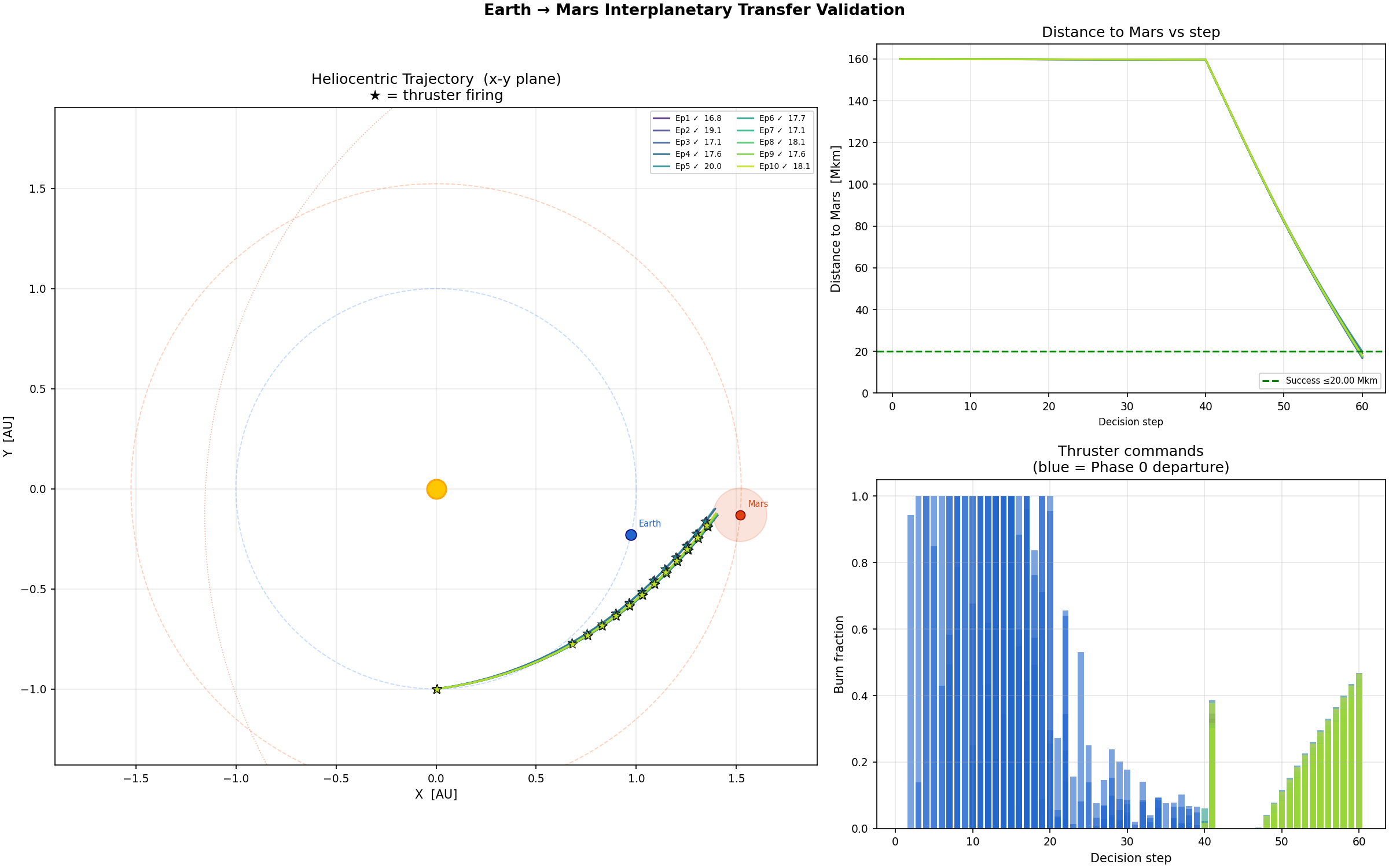
mars_v11 evaluation across 12 episodes. Heliocentric trajectory (left), distance-to-Mars curve (top right), and burn commands by phase (bottom right, blue = Phase 0 departure, green = Phase 1 corrections). All episodes arrive within the 20 Mkm sphere.
The left panel shows the heliocentric plane. Earth starts at the bottom of the frame, the spacecraft traces the lower half of a transfer ellipse, and every episode closes on Mars on the right. The distance-to-Mars curve decays monotonically from 240 Mkm at departure to between 14 and 20 Mkm at arrival. The burn command panel shows the expected two-region structure: dense blue bars during the first 20 steps as the agent executes the TMI burn in pieces within a single LEO orbit pass, then 100 steps of near-zero green bars during heliocentric coast, with small corrective pulses near the end of the episode as the spacecraft approaches Mars.
The final reward across evaluation episodes averages around 335. For reference, the v2 run that simply coasted scored near zero, v3’s unselective burning scored around 95, and v5 scored around 102 before plateauing. v11 is the first run whose policy is qualitatively doing the right thing.
06 — The 20 Mkm Wall
Every v11 evaluation episode arrives within the 20 Mkm sphere around Mars, but essentially none close to within 10 Mkm. The scatter is tight between 14 and 20. At first I tried to tune it by adjusting the Phase 1 correction cap, the proximity bonus scale, the entropy coefficient, and the network width. None of it moved the miss distance distribution by more than 1 Mkm.
The actual explanation is that the miss distance is set almost entirely by Phase 0, and Phase 1 corrections are provably incapable of removing the residual.
Cross-Track is Energy-Neutral
A cross-track burn changes the direction of the velocity vector without changing its magnitude, so the orbit’s specific energy is preserved. Specific energy determines the semi-major axis, which determines the aphelion, which determines where the transfer ellipse meets Mars’s orbit. Any miss distance that originates from an energy error in Phase 0 (overshooting or undershooting Mars’s orbital radius) is outside the set of things cross-track burns can touch. In a 2D simulation this leaves only the in-plane orientation of the orbit as a controllable degree of freedom, and the 300-second departure step quantisation sets roughly 18 to 19 Mkm of unavoidable orientation error before any cross-track burn fires.
Why Not Burn Toward Mars Instead: Earlier versions of Phase 1 tried “burn along the spacecraft-to-Mars direction” rather than cross-track. However, Mars sits roughly 9° ahead of the spacecraft’s velocity vector at arrival, so 99% of any Mars-pointed burn ends up along-track, inflates the orbital energy, and pushes the aphelion past Mars.
One-Dimensional Action Space
The agent commands a single scalar in [0, 1] and the environment picks the direction. For Phase 0 that is fine because geocentric prograde is the right direction for any departure burn. For Phase 1 it is the root of the problem. A real correction maneuver decomposes into three orthogonal components (radial, along-track, cross-track) and the optimal direction depends on where in the orbit the burn is fired. The agent has no way to express any of this. Every Phase 1 burn is forced into the single pre-selected cross-track direction regardless of what the orbit geometry actually calls for at that moment.
No Mars Orbit Insertion
The episode ends the moment the spacecraft crosses into the 20 Mkm sphere. In a real mission this is the start of the hard part: a capture burn at Mars periapsis that drops the spacecraft into a Mars-centred orbit. Without that terminal phase, the agent has no incentive to arrive at Mars with a specific velocity relative to Mars, so closing further than 20 Mkm earns nothing while spending fuel for the capture burn earns nothing either. The reward landscape has no gradient beyond the success sphere.
Hardcoded Circular Orbits
Earth and Mars are treated as idealised circular co-planar orbits at their mean heliocentric radii. Real orbits have non-zero eccentricity (Mars is at 0.0934, which moves its heliocentric distance by roughly 20 Mkm across a Mars year) and an inclination between them of roughly 1.85°. The 1.85° inclination alone contributes about 4.8 Mkm of out-of-plane distance at Mars’s orbit radius, which is a substantial fraction of the 20 Mkm success threshold. The current env simulates neither.
Where the Error Actually Comes From: Integrating the oracle’s trajectory from the moment of TMI completion shows that the residual miss distance is set to within 2 Mkm by the time the spacecraft exits Earth’s sphere of influence. The 300-second Phase 0 decision step quantises the TMI burn timing by about half an LEO orbital period divided by 40, which is a few seconds of firing error, which propagates to millions of kilometres at Mars. Closing this gap requires continuous control over the burn timing; no amount of Phase 1 correction can recover it.
07 — What Comes Next
Next week’s work is an environment rewrite rather than another hyperparameter sweep.
Phase 1 gets a multi-dimensional action space. Adding radial and along-track components alongside cross-track gives the agent actual control over the arrival geometry, and with that control the closest-approach distribution should narrow below 10 Mkm without changing anything else about the reward.
A Mars orbit insertion phase gets appended to the episode. The arrival condition becomes “captured into a Mars-centred orbit below some apoapsis” rather than “passed within 20 Mkm”. This gives the agent a reason to arrive at Mars with a controlled relative velocity, which closes the loop on the transfer.
Planet positions get pulled from an ephemeris rather than from the circular-orbit approximation. Pointing the planet state messages at real SPICE positions fixes the orbit eccentricities and the mutual inclination.
The simulator itself has always been 3D; only the initial conditions and the target geometry were restricted to the x-y plane to simplify observation design. Once the planets are on real orbits, the out-of-plane component becomes meaningful and the observation vector has to carry it.
The interesting experiment for Week 8 is whether a policy trained on the ephemeris env can still produce the same clean TMI-plus-corrections structure that v11 found, or whether real orbit geometry produces training pathologies that the idealised version hid.
Leave a Reply
You must be logged in to post a comment.