Week 5: Visualising Theory

If you somehow churned through my blogs and still kept interest, this is your reward. Today, we officially move away from the headache-inducing math, into something easily grasped: the simulation.

We’ve spent the last few weeks going over the mathematical foundation of this project, that is, deriving the governing equations, using them to formulate a state-space representation, and finally, using those matrices in our cost function and the Riccati Equation. Now, it’s time to put those theories into practice.

I’ve spent the last week learning how to use Simscape, the software used to make the simulation, and actually building it. At first, all the moving pieces and their respective ports seemed intimidating. However, after playing around with it, it became clear to me that it was no harder than building a LEGO set; you simply drag and drop the pieces, connect them, and use Rigid Transform if any of them misbehave.

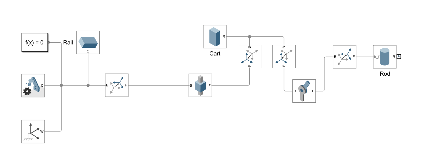
The first thing that I did was build the physical pendulum itself. I wanted to make sure that the Physics functioned as expected before I proceeded with the build. My first attempt looked something like this.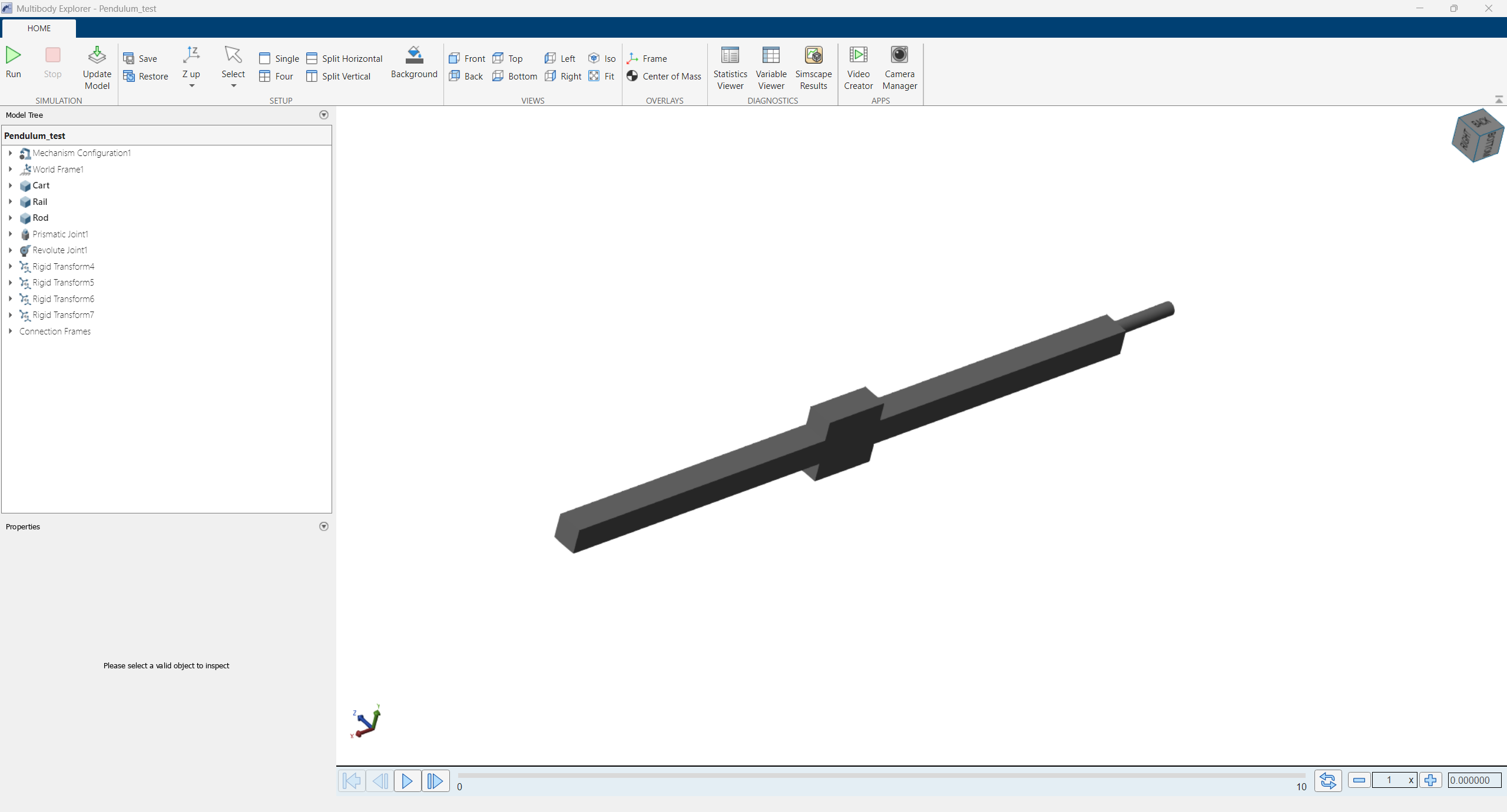Right, remember those Rigid Transforms? This is what happens when they are not properly used. I’ve also ended up with the rod sticking right out and in all directions except upright. Because of how some of the blocks (the prismatic joint) were designed, they don’t have an internal option to change their orientation, so I had to use those Rigid Transforms to get them aligned with the axis I needed.

In this form, the pendulum behaved like a physics problem, no friction, no energy loss, perfect energy conservation. In this state, letting it fall from an angle and watching it is already satisfying enough.

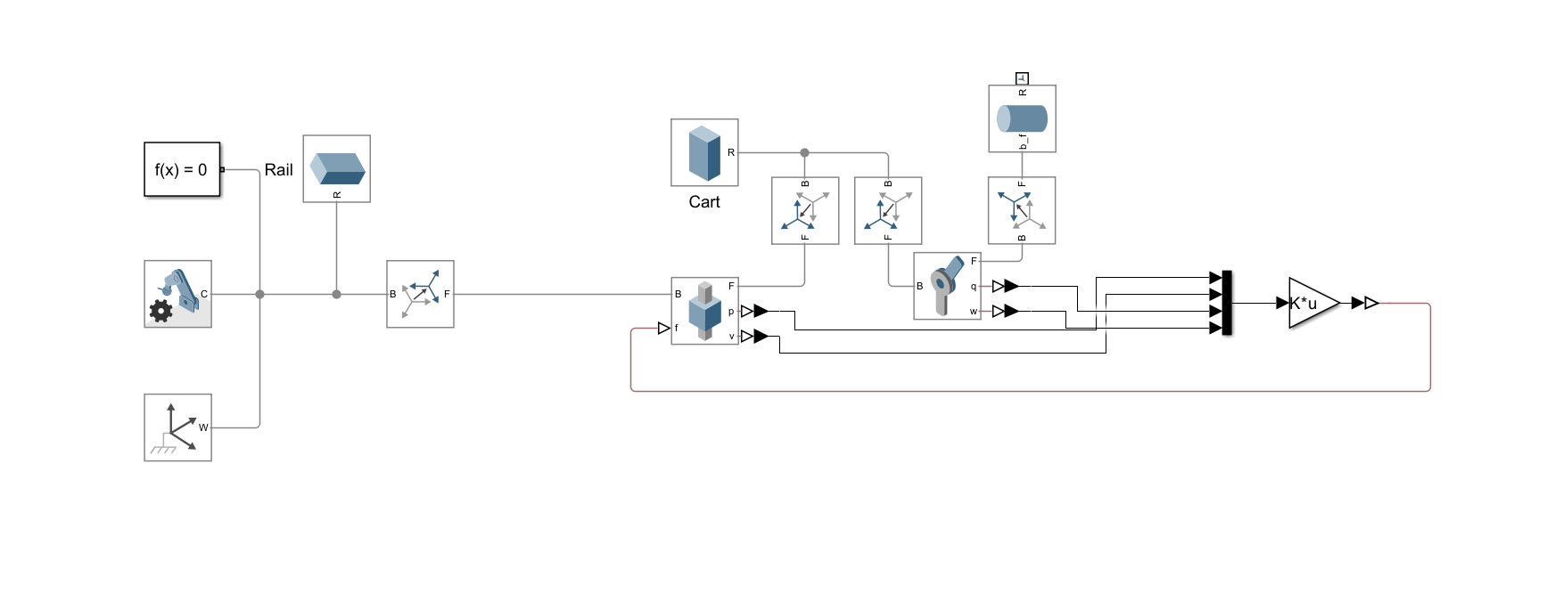
But we can do one better. By taking position and velocity outputs from the joints, we can wire the system up to our control mechanism. Remember all that math we’d been doing was in preparation for this? This is where it comes into play. Luckily, most of the numbers we crunched do not transiently evolve with the system, so the implementation is surprisingly simple.

Where K is calculated from the matrices we derived, and x is the state vector. Because our only input to the system is the force acting on the cart, we link the controller back to it.

By doing so, the inverted pendulum is now officially working.

(The kick around 5s is intentional)

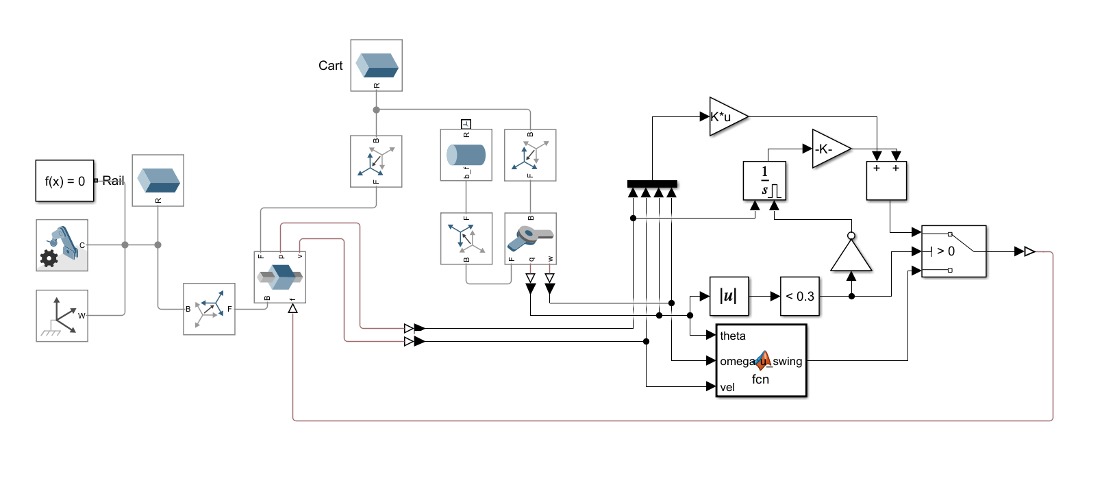
Right now, the pendulum can balance upright only when it starts upright; it can’t swing itself up from a downward position. Because we used small-angle approximations in deriving the equation, the LQR controller can only reliably restore balance over a limited range of angles around the upright position. To enable it to swing up, I added another controller, this time for energy.

It calculates the system’s current energy and compares it to the energy of the system if it were upright. If the system hasn’t gained enough energy yet, it rocks the cart back and forth until it has. Adding this gives us a very nice swing-up animation.

Under the ideal conditions of a world recreated in a computer, this has no flaws. However, in a real-world scenario, LQR will break under the slight tilt of the table, the friction of the track, and the non-ideal behavior of the encoder shaft, as a Linear Quadratic Regulator does not account for imperfections. But an LQI does. The Linear Quadratic Integral has an additional integral term compared to LQR. This allows it to recognize errors that have accumulated since the pendulum began running. For example, over time, it will note the table’s slant and apply additional force to correct that error. Adding it gives us the final version of the simulation. Functionally, it is identical to an LQR, but provides a more robust countermeasure against steady-state errors.

We have now officially finished the simulation. I am currently gathering supplies to finally build the physical pendulum. Check in next week to see the progress!